Page 387 - Pipeline Risk Management Manual Ideas, Techniques, and Resources

362 Leak Rate Determination
Liquid-the quantity of liquid released from a full-bore line upstream condition. Sonic velocity is a limiting factor for gas
rupture at MAOP (for normal operating pressure) for 1 hour flow through an orifice.
(60 minutes). An alternative approach is to model the spill
volume as the maximum pumped flowrate for a fixed time
period (perhaps based on estimated reaction times) plus the Liquid flow
volume that would be drained to the spill location.
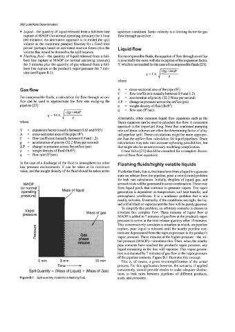
Flashingfluid-the quantity of liquid released from a full- For incompressible fluids, the equation of flow through an orifice
bore line rupture at MAOP (or normal operating pressure) is essentially the same with the exception of the expansion factor,
for 3 minutes plus the quantity of gas released from a full- Y, which is not needed for the case of incompressible fluids [23]:
bore line rupture at the product’s vapor pressure for 7 min-
Utes (see Figure B. 1). q=CA

where
Gas flow A = cross-sectional area of the pipe (e2)
C = flow coefficient (usually between 0.9 and 1.2)
For compressible fluids, a calculation for flow through an on- g = acceleration ofgravity (32.2 ft/sec per second)
fice can be used to approximate the flow rate escaping the A p = change in pressure across the orifice (psi)
pipeline [23]: p = weight density of fluid (lb/ft3)
q = YCA L- q = flow rate (ftVsec).
(2g) 144AP

where Alternately, other common liquid flow equations such as the
Darcy equation can be used to calculate this flow. A consistent
approach is the important thing. Note that continued pumping
Y = expansion factor (usually between 0.65 and 0.95) rate and drain volumes are often the determining factor of a liq-
A = cross-sectional area of the pipe (ft2) uid pipeline spill. These calculations might be more appropri-
c= ate than the orifice flow calculation for liquid pipelines. Drain
flow coefficient (usually between 0.9 and 1.2)
g = acceleration of gravity (32.2 ft/sec per second) calculations may take into account siphoning possibilities, but
AP = change in pressure across the orifice (psi) that might also be an unnecessary modeling complication.
P = weight density of fluid (lb/ft3) Crane Valve [23] should be consulted for a complete discus-
q = flow rate (ftVsec). sion of these flow equations.
In the case of a discharge of the fluid to atmosphere (or other Flashing fluidslhighly volatile liquids
low pressure environment), Y can be taken at its minimum
value, and the weight density of the fluid should be taken at the Fluids that flash, that is, that transform hm a liquid to agaseous
state on release from the pipeline, pose a complicated problem
for leak rate calculation. Initially, droplets of liquid, gas, and
aerosol mists will be generated in some combination. These may
form liquid pools that continue to generate vapors. The vapor
(oFcKal4 Mass,of liquid
ooeratina
generation is dependent on temperature, soil heat transfer, and
piessurij atmospheric conditions. It is a nonlinear problem that is not
readily solvable. Eventually, if the conditions are right, the liq-
uid will all flash or vaporize and the flow will be purely gaseous.
To simplify this problem, an arbitrary scenario is chosen to
Vapor simulate this complex flow. Three minutes of liquid flow at
pressure
MOP is added to 7 minutes of gas flow at the product’s vapor
pressure to arrive at the total release quantity after 10 minutes.
This conservatively simulates a situation in which, on pipeline
p!
pure
3 r~pt~~, liquid is released until the nearby pipeline con-
CD
CD tents are depressured from the rupture pressure to the product’s
!+!
a vapor pressure. Three minutes at the higher pressure-the ini-
tial pressure (MAOPHimulates this. Then, when the nearby
pipe contents have reached the product’s vapor pressure, any
liquid remaining in the line will vaporize. This vapor genera-
Time - of the pipeline contents. Figure B. 1 illustrates this concept.
tion is simulated by 7 minutes of gas flow at the vapor pressure
0 min 3 rnin 10 rnin process. For this application however, the scenario, if applied
This is, of course, a gross oversimplification of the actual
Spill Quantity = (Mass of Liquid) + (Mass of Sas) consistently, should provide results to make adequate distinc-
tions in leak rates between pipelines of different products,
Figure B.1 Spill quanti model for a flashing fluid. sizes, and pressures.