Page 517 - Pipelines and Risers

484 Chapter 25

Ph= Probability of failure in yearn

In this calculation example the inflation rate used is 2% and the "interest rate" used is 6%.
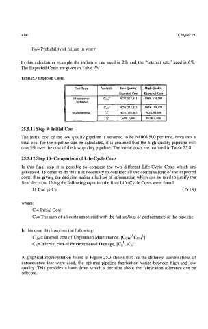
The Expected Costs are given in Table 25.7.

Table25.7 Expected Costs.

Envimental I &" I NOK129.363 I NOK94.490 [

25.5.11 Step 9- Initial Cost

The initial cost of the low quality pipeline is assumed to be NOK6,500 per tone, from this a
total cost for the pipeline can be calculated, it is assumed that the high quality pipeline will
cost 5% over the cost of the low quality pipeline. The initial costs are outlined in Table 25.8

25.5.12 Step 10- Comparison of Life-Cycle Costs
In this final step it is possible to compare the two different Life-Cycle Costs which are
generated. In order to do this it is necessary to consider all the combinations of the expected
costs, thus giving the decision maker a full set of information which can be used to justify the
final decision. Using the following equation the final Life-Cycle Costs were found:
LCC=C,+ CF (25.19)

where:
CI= Initial Cost
CF The sum of all costs associated with the failureAoss of performance of the pipeline

In this case this involves the following:
CUM= Interval cost of Unplanned Maintenance, [C~hn",Cm~]
CE= Interval cost of Environmental Damage, [CE", CE"]

A graphical representation found in Figure 25.3 shows that for the different combinations of
consequence that were used, the optimal pipeline fabrication varies between high and low
quality. This provides a basis from which a decision about the fabrication tolerance can be
selected.