Page 142 - Power Electronic Control in Electrical Systems

//SYS21/F:/PEC/REVISES_10-11-01/075065126-CH004.3D ± 130 ± [106±152/47] 17.11.2001 9:54AM

130 Power flows in compensation and control studies

4.4.5 Numerical example 3

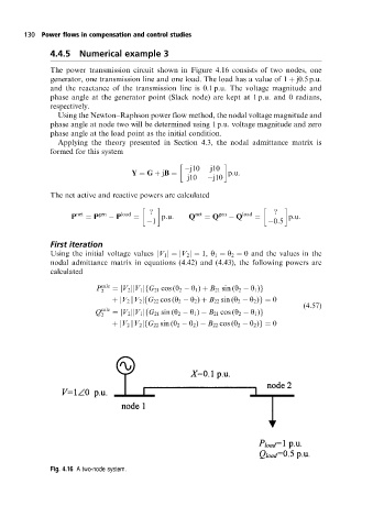
The power transmission circuit shown in Figure 4.16 consists of two nodes, one
generator, one transmission line and one load. The load has a value of 1 ‡ j0:5p:u:
and the reactance of the transmission line is 0.1 p.u. The voltage magnitude and
phase angle at the generator point (Slack node) are kept at 1 p.u. and 0 radians,
respectively.
Using the Newton±Raphson power flow method, the nodal voltage magnitude and
phase angle at node two will be determined using 1 p.u. voltage magnitude and zero
phase angle at the load point as the initial condition.
Applying the theory presented in Section 4.3, the nodal admittance matrix is
formed for this system

j10 j10
Y ˆ G ‡ jB ˆ p:u:
j10 j10
The net active and reactive powers are calculated

? net gen load ?
gen
load
net
P ˆ P P ˆ p:u: Q ˆ Q Q ˆ p:u:
1 0:5
First iteration
Using the initial voltage values V 1 j ˆ V 2 j ˆ 1, y 1 ˆ y 2 ˆ 0 and the values in the
j
j
nodal admittance matrix in equations (4.42) and (4.43), the following powers are
calculated
P calc ˆ V 2 kV 1 j G 21 cos (y 2 y 1 ) ‡ B 21 sin (y 2 y 1 )g
f
j
2
‡ V 2 kV 2 j G 22 cos (y 2 y 2 ) ‡ B 22 sin (y 2 y 2 )g ˆ 0
j
f
(4:57)
Q calc ˆ V 2 kV 1 j G 21 sin (y 2 y 1 ) B 21 cos (y 2 y 1 )g
j
f
2
‡ V 2 kV 2 j G 22 sin (y 2 y 2 ) B 22 cos (y 2 y 2 )g ˆ 0
f
j

Fig. 4.16 A two-node system.