Page 139 - Power Electronic Control in Electrical Systems

//SYS21/F:/PEC/REVISES_10-11-01/075065126-CH004.3D ± 127 ± [106±152/47] 17.11.2001 9:54AM

Power electronic control in electrical systems 127

n
X
P l ˆjV l j jV m jfG lm cos (y l y m ) ‡ B lm sin (y l y m ) (4:42)
m ˆ 1
n
X
Q l ˆjV l j jV m jfG lm sin (y l y m ) B lm cos (y l y m ) (4:43)
m ˆ 1
where jV l j and jV m j are the nodal voltage magnitudes at nodes l and m and y l and y m
are the nodal voltage phase angles at nodes l and m.
These equations provide a convenient device for assessing the steady state beha-
viour of the power network. The equations are non-linear and their solution is
reached by iteration. Two of the variables are specified while the remaining two
variables are determined by calculation to a specified accuracy. In PQ type nodes two
equations are required since the voltage magnitude and phase angle jV l j and y l are
not known. The active and reactive powers P l and Q l are specified. In PV type nodes
one equation is required since only the voltage phase angle y l is unknown. The active
power P l and voltage magnitude jV l j are specified. For the case of the Slack node
both the voltage magnitude and phase angle jV l j and y l are specified, as opposed to
being determined by iteration. Accordingly, no equations are required for this node
during the iterative step.
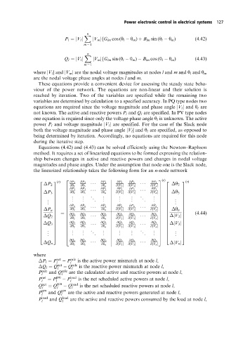
Equations (4.42) and (4.43) can be solved efficiently using the Newton±Raphson
method. It requires a set of linearized equations to be formed expressing the relation-
ship between changes in active and reactive powers and changes in nodal voltage
magnitudes and phase angles. Under the assumption that node one is the Slack node,
the linearized relationship takes the following form for an n-node network

3 (r) 2 3 (r) 2 3 (r)
2 @P 2 @P 2 @P 2 @P 2 @P 2 @P 2
P 2 y 2
@y 2 @y 3 @y n @jV 2 j @jV 3 j @jV n j
6 @P 3 @P 3 @P 3 @P 3 @P 3 @P 3 7
6 7 6 7
6 7
@y 2 @y 3 @y n @jV 2 j @jV 3 j @jV n j
6 P 3 7 6 y 3 7
6 7
6 7 . . . . . . . 6 7
. 6 . . . . . . . . . 7 .
6 . 7 6 . . . . . . . . 7 6 . 7
6 . 7 6 7 6 . 7
6 7 6 7
@P n @P n @P n @P n @P n
6 @P n 7

6 7 6 7
@y 2 @y 3 @y n @jV 2 j @jV 3 j @jV n j
6 7
6 P n 7 6 y n 7
6 7 (4:44)
6 7 6 7
@Q 2 @Q 2 @Q 2 @Q 2 @Q 2 @Q 2 7
ˆ 6
6 Q 2 7 6 jV 2 j 7
@y 2 @y 3 @y n @jV 2 j @jV 3 j @jV n j
6 7
6 7 6 7
6 7
6 7 6 7
@Q 3 @Q 3 @Q 3 @Q 3 @Q 3

6 @Q 3 7
6 Q 3 7 6 jV 3 j 7
@y 2 @y 3 @y n @jV 2 j @jV 3 j @jV n j 7
6
6 7 6 7
. 6 . . . . . . . 7
6 . 7 6 . . . . . . . . . 7 6 . 7
6 . 7 6 . . . . . . . . 7 6 . . 7
4 5 4 5
4 5
@Q n @Q n @Q n @Q n @Q n @Q n
Q n jV n j
@y 2 @y 3 @y n @jV 2 j @jV 3 j @jV n j
where
P l ˆ P net P calc is the active power mismatch at node l,
l
l
Q l ˆ Q net Q calc is the reactive power mismatch at node l,
l
l
P calc and Q calc are the calculated active and reactive powers at node l,
l
l
P net ˆ P gen P load is the net scheduled active powers at node l,
l
l
l
Q net ˆ Q gen Q load is the net scheduled reactive powers at node l,
l
l
l
P gen and Q gen are the active and reactive powers generated at node l,
l
l
P load and Q load are the active and reactive powers consumed by the load at node l,
l l