Page 152 - Practical Control Engineering a Guide for Engineers, Managers, and Practitioners

Matrices and Higher- 0 r de r Process Mode Is 127

For this particular process the vectors and matrices occurring in
Eq. (5-8) are

0 0
rt ~
X=[~ :l A= R, 1 r2 0 B= rt U = F 0
0
RI r2
RJ _!_ 0
0
R r rJ
2 3
c = (0 0 1) Y= XJ
Here, the process input ll has one element that is presented to the
model via the column vector B. The process output Y has one element
that is extracted from the state \·ector via the row vector C. The state
of the process X has three elements. This is called the state-space
approach to presenting the process model.
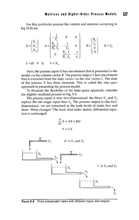
To illustrate the flexibility of the state-space approach, consider
the slightly modified process in Fig. 5-4
The process input is now two-dimensional: the flows VI and v2
replace the old single input flow F • The process output is also rn·o-
0
dimensional. ·we are interested in the tank levels of tanks rn'o and
three. What changes? The basic first-order matrix differential equa-
tion is unchanged:

.!!_X= AX+ BU
dt
Y=CX
r=v,

+
jx, ~v
L_--~==~~ ~ 2

I I x,

f,
~-

1

F1ouRE 5-4 Three independent tanks with different inputs and outputs.