Page 196 - Practical Control Engineering a Guide for Engineers, Managers, and Practitioners

170 Chapter Six

which can be solved for KY, KY,, and Ku as in

(6-14)

This completes the construction of the modified process. There is
one nontrivial problem remaining-how does one get values of
dy / dx or y' so it can be fed back? For the time being we will assume
that y' is available by some means. In Chap. 10, the Kalman filter will
be shown as one means of obtaining estimates of y and y' or, in gen-
eral, the state of the process, especially in a noisy atmosphere. Alter-
natively, we might try generating dy I dt or y' by using a filtered
differentiator in a manner similar to what was used in generating the
PID single in the Sec. 6-4.
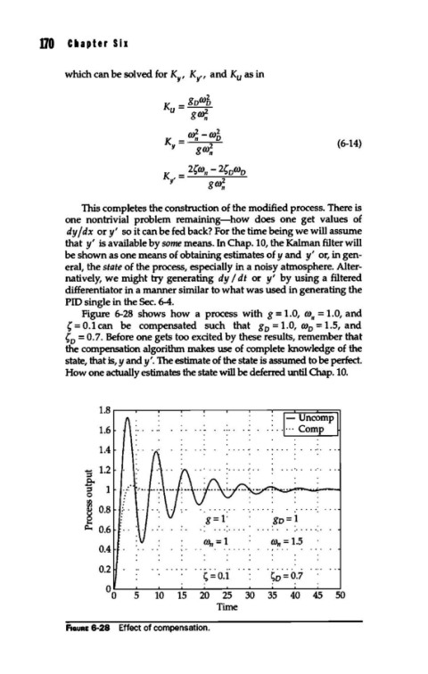
Figure 6-28 shows how a process with g = 1.0, co,= 1.0, and
{ = 0.1 can be compensated such that g = 1.0, co = 1.5, and
0 0
{ = 0.7. Before one gets too excited by these results, remember that
0
the compensation algorithm makes use of complete knowledge of the
state, that is, y andy'. The estimate of the state is assumed to be perfect.
How one actually estimates the state will be deferred until Chap. 10.

1.8 r----r---r--~-~----.-..,....-----,.----r:=:::::t:;:;:==:J=::::;,

1.6
1.4
::s 1.2
t 1
0
Ia .....
(U 0.8
e g=1: .Ko=~
Q... 0.6 . . .....
co,= 1 co,= 1.5
0.4 \. . .....
0.2 ...... " . .....
~=0.1 ~o=0.7
00 5 10 15 20 25 30 35 40 45 50
Time

F1auRE 6-28 Effect of compensation.