Page 193 - Practical Control Engineering a Guide for Engineers, Managers, and Practitioners

An Underdamped Process 167

Remember that the s operator takes the derivative of what fol-
2
lows it. Solving Eq. (6-9) for the second derivative of y, namely s y(s)
2
2
or d y/dt or y", gives
2
s y(s) = -2{ron s y(s)- ro~ y(s) + gro; ii(s) (6-10)
In the time domain, Eq. (6-10) would look like

Note that ron and g have reappeared but remember that t and y
can always be scaled to make both quantities unity.
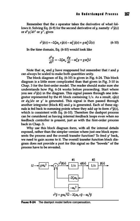
The block diagram of Eq. (6-10) is given in Fig. 6-24. This block
diagram is a little more complicated than that given in Fig. 3-10 in
Chap. 3 for the first-order model. The reader should make sure she
understands how Fig. 6-24 works before proceeding. Start where
2
you see s y(s) in the diagram. This signal passes through one inte-
grator represented by the #1 block containing 1/s. As a result, sy(s)
or dyfdx or y' is generated. This signal is then passed through
another integrator (block #2) and y is generated. Each of these sig-
2
nals is fed back to summing points where they add up to form s y(s),
which is consistent with Eq. (6-10). Therefore the dashpot process
can be considered as having internal feedback loops even when no
feedback controller is present, just as with the first-order process
back in Chap. 3.
Why use this block diagram form, with all the internal details
exposed, rather than the simpler version where just one block repre-
sents the process and the overall transfer function? To feed y' back,
we need to gain access to it. The overall transfer function block dia-
gram does not provide a port for this signal so the ''bowels" of the
process have to be revealed.

#1 #2
y(s)
u

F1auRE 6-24 The dashpot model before compensation.