Page 189 - Practical Control Engineering a Guide for Engineers, Managers, and Practitioners

164 Chapter Six

~ 2.5
~ 2
o.._ 1.5
"''::S
;.& 1 ----- .. · - · Set point . .
- ;:::s . . .. - Process output : . .
.s 0 0.5
0
0.. 0 . . . . . . . . . . . . . . . . . ..
~ -0.50
10 20 30 40 50 60 70 80 90 100
8
'E
.& 6 . . . . . . . ... . . . .
5
.... 4
~ 2 ~;
~
c 0~·
0
u
-2
0 10 20 30 40 50 60 70 80 90 100
Tune
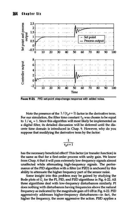
fiGURE 6-21. PlfD set-point step-change response with added noise.

Note the presence of the 1 I ( r s + 1) factor in the derivative term.
0
For our simulation, the filter time constant r 0 was chosen to be equal
to 1 I co, = 1. Since this algorithm will most likely be implemented as
a digital filter, its detailed discussion will be deferred until the dis-
crete time domain is introduced in Chap. 9. However, why do you
suppose that modifying the derivative term by the factor:

has the necessary beneficial effect? This factor (or transfer function) is
the same as that for a first-order process with unity gain. We know
from Chap. 4 that it will pass extremely low-frequency signals almost
unaffected while attenuating high-frequency signals. The perfor-
mance of the PID algorithm with a filter (or PlfD) is anchored by this
ability to attenuate the higher frequency part of the sensor noise.
Some insight into this problem may be gained by studying the
Bode plots of Gc for the PI, PID, and PlfD algorithms in Fig. 6-22. All
three algorithms deal with low-frequency disturbances similarly. PI
does nothing with disturbances having frequencies above the natural
frequency as indicated by the magnitude gain of 0 dB in Fig. 6-22. PID
aggressively addresses higher-frequency disturbances-in fact, the
higher the frequency, the more aggressive the action. PlfD applies a