Page 188 - Practical Control Engineering a Guide for Engineers, Managers, and Practitioners

11 llllerll••~tell Precess 113

I 25~--~----~-----r----~----~--~
2

1i 1~ •••••• . . ········'·················
l 0.: :.:::::t:::::::l::::::::J~~-~~.1:::::::
0
i ~~ ro ~ ~ ~ ~ M

10
~
j.
g 5
...
&
I 0
u

Tune
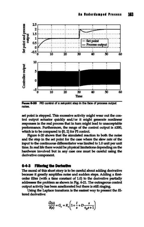
Aa .. 8-20 PID control of a set-point step In the face of process output
noise.

set point is stepped. This excessive activity might wear out the con-
trol output actuator quickly and/ or it might generate nonlinear
responses in the real process that in tum might lead to unacceptable
performance. Furthermore, the range of the control output is ±200,
which is to be compared to [0, 2] for PI controL
Figure 6-20 shows that the simulated reaction to both the noise
and the step in the set point for the case where the slew rate of the
input to the continuous differentiator was limited to 1.0 unit per unit
time. In real life there would be physical limitations depending on the
hardware involved but in any case one must be careful using the
derivative component.

8-4-3 RlterlnJ tile Derivative
The moral of this short story is to be careful about adding derivative
because it greatly amplifies noise and sudden steps. Adding a first-
Older filter (with a time constant of 1.0) to the derivative partially
addresses the problem as shown in Fig. 6-21. The outrageous control
output activity has been ameliorated but there is still ringing.
Using the Laplace transform is the easiest way to present the fil-
tered derivative:

U(s) ( I s )
_() =Gc: =Kc: 1+-+D--
e s s -r s+ 1
0