Page 190 - Practical Control Engineering a Guide for Engineers, Managers, and Practitioners

An Underdamped Process 165

.. ·
.. : :· ..
&i 60
:2-
QJ 40
"'0 · .. ·
.a .. ··.
·~ 20 f. ·:···. :. • •• ' •• • ,
ns . -....... ::;_,,:.:~-·- ·-:-·-· ~ ·-·-:-·- ..... -·:.
:E 0 ,

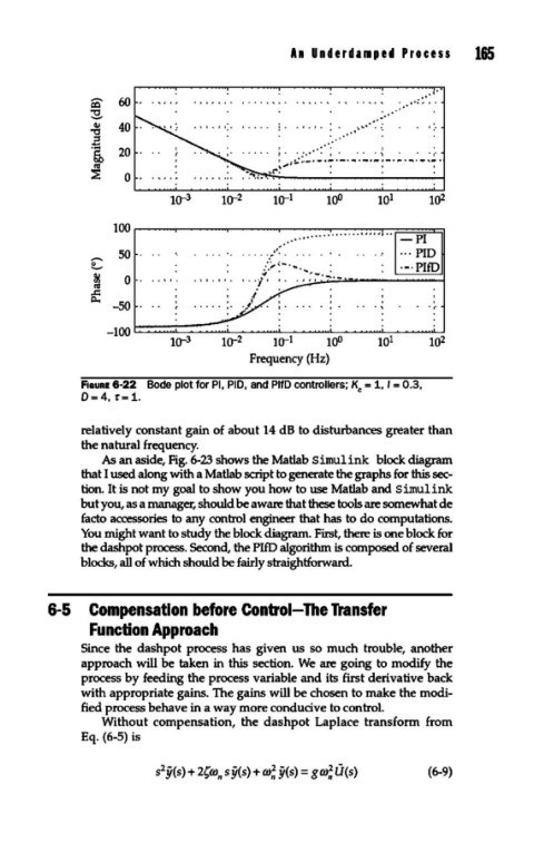
F1auRE 6-22 Bode plot for PI, PI D. and PlfD controllers; Kc = 1, I= 0.3,
0=4, T=1.

relatively constant gain of about 14 dB to disturbances greater than
the natural frequency.
As an aside, Fig. 6-23 shows the Matlab simulink block diagram
that I used along with a Matlab script to generate the graphs for this sec-
tion. It is not my goal to show you how to use Matlab and simulink
but you, as a manager, should be aware that these tools are somewhat de
facto accessories to any control engineer that has to do computations.
You might want to study the block diagram. First, there is one block for
the dashpot process. Second, the PlfD algorithm is composed of several
blocks, all of which should be fairly straightforward.

6-5 Compensation before Control-The Transfer
Function Approach
Since the dashpot process has given us so much trouble, another
approach will be taken in this section. We are going to modify the
process by feeding the process variable and its first derivative back
with appropriate gains. The gains will be chosen to make the modi-
fied process behave in a way more conducive to control.
Without compensation, the dashpot Laplace transform from
Eq. (6-5) is

(6-9)