Page 198 - Practical Control Engineering a Guide for Engineers, Managers, and Practitioners

172 Chapter Six

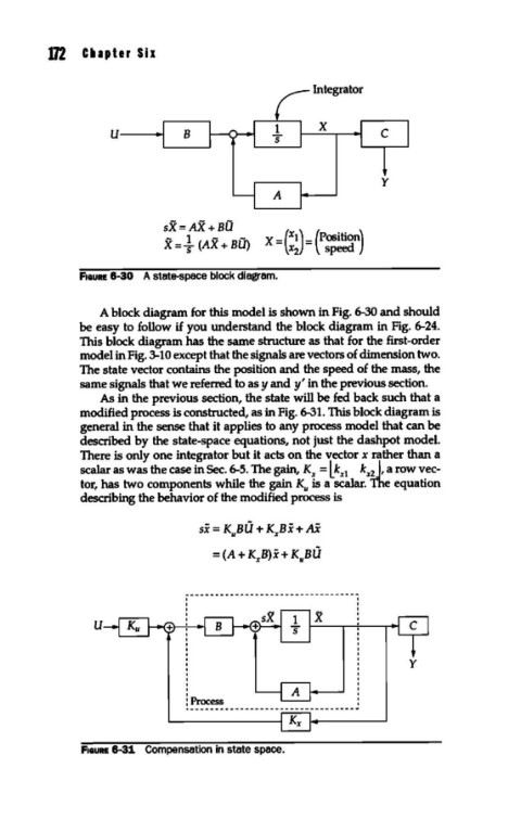
sX=AX+BU
- 1 - - X= (xt) = (Position)
X= 5 (AX+BU) x 2 speed)

FIGURE 8-30 A state-space block diagram.

A block diagram for this model is shown in Fig. 6-30 and should
be easy to follow if you understand the block diagram in Fig. 6-24.
This block diagram has the same structure as that for the first-order
model in Fig. 3-10 except that the signals are vectors of dimension two.
The state vector contains the position and the speed of the mass, the
same signals that we referred to as y and y' in the previous section.
As in the previous section, the state will be fed back such that a
modified process is constructed, as in Fig. 6-31. This block diagram is
general in the sense that it applies to any process model that can be
described by the state-space equations, not just the dashpot model.
There is only one integrator but it acts on the vector x rather than a
scalar as was the case in Sec. 6-5. The gain, Kx = l kxt kx I, a row vec-
2
tor, has two components while the gain K" is a scalar. The equation
describing the behavior of the modified process is

si = K"BU + KxBi+ Ai

=(A+ KXB)i+ KUBU

u

y

~------------~ Kx
FIGURE 8-31. Compensation in state space.