Page 210 - Practical Control Engineering a Guide for Engineers, Managers, and Practitioners

184 Chapter Seven

So, we have solved Eq. (7-9) for the spatial dependence of the
temperature with the Laplace transforms as a parameter. Alterna-
tively, we could look at Eq. (7-10) as the Laplace transform of T{z,t)
with the spatial dimension z as a parameter.

7-3-1 Inlet Temperature Transfer Function
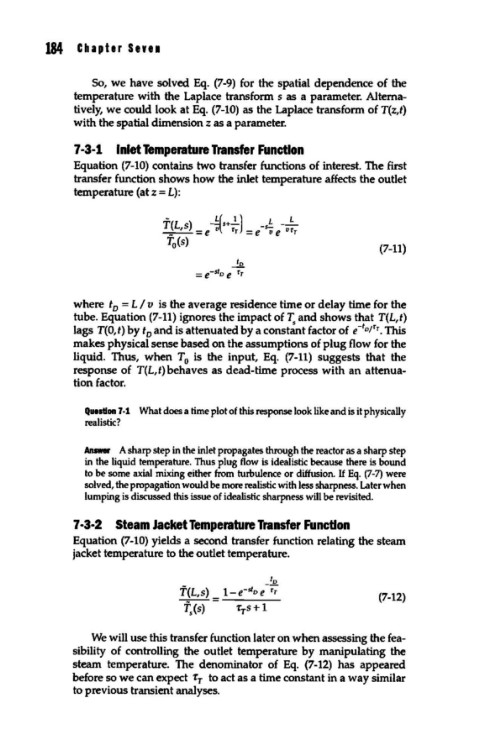
Equation (7-10) contains two transfer functions of interest. The first
transfer function shows how the inlet temperature affects the outlet
temperature (at z = L):

T(L s) - L( s+..!..) L -....!::....
---'- = t V\. rT = t -SV t vrT
T (s)
0 (7-11)

where t = L I v is the average residence time or delay time for the
0
tube. Equation (7-11) ignores the impact of~ and shows that T(L,t)
1
lags T(O,t) by t and is attenuated by a constant factor of e- v/rT. This
0
makes physical sense based on the assumptions of plug flow for the
liquid. Thus, when T is the input, Eq. (7-11) suggests that the
0
response of T(L,t) behaves as dead-time process with an attenua-
tion factor.
Question 7-1 What does a time plot of this response look like and is it physically
realistic?
Answer A sharp step in the inlet propagates through the reactor as a sharp step
in the liquid temperature. Thus plug flow is idealistic because there is bound
to be some axial mixing either from turbulence or diffusion. U Eq. (7-7) were
solved, the propagation would be more realistic with less sharpness. Later when
lumping is discussed this issue of idealistic sharpness will be revisited.

7-3-2 Steam Jacket Temperature Transfer Function
Equation (7-10) yields a second transfer function relating the steam
jacket temperature to the outlet temperature.

to
f(L,s) _ 1- e-sto e -r;
(7-12)
T(s) - -r s + 1
1
5
We will use this transfer function later on when assessing the fea-
sibility of controlling the outlet temperature by manipulating the
steam temperature. The denominator of Eq. (7-12) has appeared
before so we can expect T 1 to act as a time constant in a way similar
to previous transient analyses.