Page 224 - Practical Design Ships and Floating Structures

199

TABLE 1
NUMERICAL DATA FOR COMBINED MODEL

Breadth B
Lineardcnsltyofmnbody pe 3 713 IO kgh
Horizontal bending ngdity EI I 090 IO Nm
Shearing ngdity k CA 2377 in Nm

Distanceofthemarntlngpointof 845 37 50 6655 m
foundation spnng (xl,2,3)
Spnngngidity(kl,Z,3) XI08 934 1149 1934 N/m
Height of dolphin H 22 5 m
Penehahon depth h 75 0 m
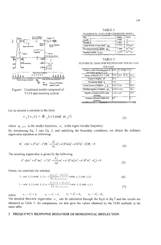
+ + PanhmdDdphur,
-4% .4&qkiLmd3 Linear density of dolphin A , 5 62 X IO4 hdm
Figure1 Combined model composed of Bendingngidityofdolphin EI, 6 70X 1013 Nm 2
VLFS and mooring system Rigdity of fendcr rod for weak I 35 x I07 Nlm
moonng
Clearance behwen fender and 0 4 m
StrUCbve

Let us assume a solution in the form
Vi(X,t) = 0 j(x)cos( wit)
(3)

where Q, , (x) is the modes functions, wI is the eigen circular frequency.
By introducing Eq. 3 into Eq. 2, and satisfying the boundary conditions, we obtain the ordinary
eigenvalue equation as following

The resulting eigenvalue is given by the following
k4
a4 +[(a2 +p2)w: -r2]a2 -(+w; +a2PZw~w~ -a2p2~; -k;)=o
w0 (5)
Hence, we conclude the solution
I 2 2 1 1 1
I-cos( l,L)cosh( L,L)=(L1s2s3 -L2sis4 ) sinh( L, L ) sin( 1, L)
2L,l*s, SIS3S4
I-cos( L,L)W)S( L,L)=( ' ) sin( L L ) sin( t I L )
/I*s2s* + n:s:s:
2l,L*st SlS3SI
where = A: + 6, s2 = A: - 6, s3 = a: + 6, s4 = a: -6,
The detailed theoretic eigenvalue o can be calculated through the Eq.6 or Eq.7 and the results are
tabulated in Table 3. As comparison, we also give the values obtained by the FEM methods in the
same table.

3 FREQUENCY RESPONSE BEHAVIOR OF HORIZONTAL DEFLECTION