Page 264 - Practical Design Ships and Floating Structures

239

OVERVIEW OF SIMLAB
SIMLAB is a general stochastic finite element system that integrates the nonlinear finite element code,
DYNA3D, into a simulation based probabilistic analysis framework. Both random sampling and Latin
Hypercube sampling techniques are used to generate random variables and random processes. The key
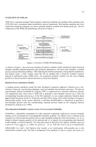
components of the SIMLAB methodology are given in Figure 1.
Most Probable Fatlure I, rl Random Problem Parameten (4) I Simulation Module

Select:

Random Process Discretization
I OUier Loop: I Loop Over Random
Process Realizations
inner Loop:
1 - DireCtRandom Uodate Finite Element lnout t
Variable Simulation
Anal sis Via the DYNA3D Solver
0"tp"t: Structural Dynamic Response Direct Random
Limit
of
via
Function
Location Failure Evaluation Accumulation State I-function
Response Uncertainty
Distribution -
Figure 1 : Overview of SIMLAB Methodology
As shown in Figure 1, the outer loop simulates all random variables which characterize basic structural
strength variables (material properties and geometric parameters). The inner loop simulates a random
process (seaway/slamming loading). After selecting the material properties, hull geometric parameters,
and applied loads, a finite element input file will be updated and a structural dynamic response
analysis is performed using a FEM solver. The maximum response variable over the entire loading
period at a critical location is stored and used in a limit state function.
Random Process Simulation Module

A random process simulation model has been developed to generate stationary Gaussian (gcs), non-
stationary Gaussian, non-Gaussian stationary, and non-Gaussian non-stationary processes. The spectral
representation method developed by Grigoriu (1 993) is employed for a Gaussian stationary process.
Two approaches have been used in SIMLAB to generate a non-Gaussian process (gNG) from the
corresponding Gaussian process (gc). In the first approach, we use a single parameter (random phase
angle) based simulation model by Shinozuka and Jan (1972), along with a small number of frequency
discretization points. In the second approach, a nonlinear transformation is introduced to generate a
non-Gaussian process from the corresponding Gaussian process based on the mapping function
developed by Sarkani et al. (1994).

Time Dependent Reliability Analysis via the First-Excursion Probability
Probabilistic vulnerability assessment of a ship structural component subjected to extreme dynamic
loading can be formulated as a time-dependent reliability problem. The failure event is defined as the
crossing of a critical response quantity above a safe threshold during the entire time history. Let s(t, y)
denote a critical response quantity of the structure and r(t, y) denote the corresponding safe threshold
(yield strength, or critical moment). The limit-state function defined in the random variables space 0)
is given by G(y) = in w(t, y). where w(t, y)=r(t, y) - s(t, y). Note that even if w(t, y) is continuously
[?o.h]
differentiable in y and t, the function G(yl usually is not continuously differentiable due to the
minimization operator used. The lack of uniqueness of the gradient of G(y) at a point will result in a