Page 84 - Pressure Swing Adsorption

,,
,, .
58 PRESS I iRE SWING ADSORPTION FUNDAMENTALS OF ADSORPTION 59
Table 2.10. Mathematical Model for an Adsorption Column
LO
·'-',~~
Differc,111;11
h.ilanct" for - - fJ= 0.713
0.8 ,
fluid phase: "'¾,.
':,__
•'I'
D!. = 0 fnr plug Jlow: ii = 0 for trace .svsiem
0.6
,1T '[ ('-') ]"T ,= 7.5
Heat baiance: l'Cgilz + cg+ -,- Cs iii c/co
. '
0.4
= (-illll( ! -. ')'1q - 4h(T- 'f) 7 ' - --
F rlt --;"J 0
Initial conditions: Adsorption, ij(z,0)=0, c(O,t)=O: 1/ - - --
Desorpt10n, ij(z,0) = q 0 , c(0,1) = 0 0.2 1/
1/
Equilibnum: Linear. q* = Kc:. Langmuir,
l. Linear rate modeis 2. Solid diffusion .,_ Pore diffusion
0.8
a. Fluid film resistance
ii(! 3kr ,. cJc rlZi
aj"=y(c-c) Ep J/ + (\ - Er,)7it 0.6
"
= €~" :n(R2~#) clco
0.4
L D,, = constant DP constunt
ii. D~ = Du(! - q/t/5)- 1
b. Solid film res1slance
0.2
,l(/
7ii. = k(q• - ij) q(r,O) = Oor,1 0 [j{r, 0) = 0 or lfo ---
q(r,:, i - z/v) = q*(z, t) ij(Rr,. f -- z/1·) = q*(z, r)
ilq 8q
a,W,t-z/u)=O aRW,t) - 0 ,
,
2
li=q= l.Jr"qr dr - ii= - 3 f "'1 l;(l ~f:o )
,;.' 0 R~ o · ' / C= 15
2
+tpc!R dR '
' '
'
clco '
0.4
an addit10nal differentml equation with associated boundary conditions. For ' '
many different boundary conditions diffusion"controllect kinetics may be
satisfactorily represented by the so"called "linear driving force" (LDF) ex- 0.2
pression:
(2.57)

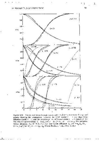
where k ~ 15D,/R 2 The validity of tlus approx1mauon, first mtroduced by Figure 2.25 Thcorct1c1.1l breakthrough curvt..:s calculated for a nonlinear O ,;ingmuH)
system showmg the comparison between the LDF model (--), the macropore
Glueckauf, 52 has been confirmed for many different mit1al and boundary diffusion model(----), and the mtracrvsiallinc diffus1on ·model (--·),based 011 the
conditions. Its applicability to a snnple Langmuir system is illustrated m Glueckauf approximation. k = l5De / R , r =kt, { = kq :z0 - d_/ cl'<.'w For mtracrvs-
2
0
2
Figure 2.25. It ,s evident that with the time constant defined in an appropn- talline diffusmn De/R =Dc/1}; for mncropore diff\ls1on De/R-=EPDl'/lEP+
0
ate manner, the LDF approximation provides a reasonable prediction of the (1-Er>)dq*/dclR!. {3= 1-q /qs. (From Ruthven,t with oernuss1onJ
breakthrough curves over a wide range of conditions. It 1s at its best when the