Page 502 - Probability and Statistical Inference

10. Bayesian Methods 479

10.2 Prior and Posterior Distributions

The unknown parameter itself is assumed to be a random variable having
its pmf or pdf h(θ) on the space Θ. We say that h(θ) is the prior distribution
of v. In this chapter, the parameter will represent a continuous real valued
variable on Θ which will customarily be a subinterval of the real line ℜ. Thus
we will commonly refer to h(θ) as the prior pdf of .
The evidence about v derived from the prior pdf is then combined with
that obtained from the likelihood function by means of the Bayes’s Theorem
(Theorem 1.4.3). Observe that the likelihood function is the conditional joint
pmf or pdf of X = (X , ..., X ) given that = θ. Suppose that the statistic T is
n
1
(minimal) sufficient for θ in the likelihood function of the observed data X
given that = θ. The (minimal) sufficient statistic T will be frequently real
valued and we will work with its pmf or pdf g(t; θ), given that v = θ, with t ∈
Τ where T is an appropriate subset of ℜ.
For the uniformity of notation, however, we will treat T as a continuous
variable and hence the associated probabilities and expectations will be writ-
ten in the form of integrals over the space T. It should be understood that
integrals will be interpreted as the appropriate sums when T is a discrete
variable instead.
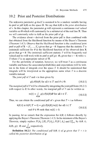
The joint pdf of T and v is then given by

The marginal pdf of T will be obtained by integrating the joint pdf from (10.2.1)
with respect to θ. In other words, the marginal pdf of T can be written as

Thus, we can obtain the conditional pdf of v given that T = t as follows:

In passing, let us remark that the expression for k(θ; t) follows directly by
applying the Bayes’s Theorem (Theorem 1.4.3). In the statement of the Bayes’s
Theorem, simply replace by k(θ; t),

h(θ), g(t; θ) and respectively.
Definition 10.2.1 The conditional pdf k(θ; t) of given that T = t is
called the posterior distribution of .