Page 506 - Probability and Statistical Inference

10. Bayesian Methods 483

Gamma(α, β) where α(> 0) and β(> 0) are known numbers. From (10.2.2),
for t ∈ T, we then obtain the marginal pmf of T as follows:

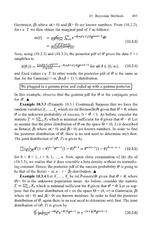
Now, using (10.2.3) and (10.3.3), the posterior pdf of given the data T = t
simplifies to

and fixed values t ∈ T. In other words, the posterior pdf of is the same as
that for the Gamma(t + α, β(nβ + 1) ) distribution.
–1
We plugged in a gamma prior and ended up with a gamma posterior.

In this example, observe that the gamma pdf for is the conjugate prior
for . !
Example 10.3.3 (Example 10.3.1 Continued) Suppose that we have the
random variables X , ..., X which are iid Bernoulli(θ) given that = θ, where
n
1
is the unknown probability of success, 0 < < 1. As before, consider the
statistic which is minimal sufficient for θ given that = θ. Let
us assume that the prior distribution of on the space Θ = (0, 1) is described
as Beta(α, β) where α(> 0) and β(> 0) are known numbers. In order to find
the posterior distribution of , there is no real need to determine m(t) first.
The joint distribution of ( , T) is given by

for 0 < θ < 1, t = 0, 1, ..., n. Now, upon close examination of the rhs of
(10.3.5), we realize that it does resemble a beta density without its normaliz-
ing constant. Hence, the posterior pdf of the success probability is going to
be that of the Beta(t + α, n – t + β) distribution. !
Example 10.3.4 Let X , ..., X be iid Poisson(θ) given that = θ, where
1
n
(> 0) is the unknown population mean. As before, consider the statistic
which is minimal sufficient for θ given that = θ. Let us sup-
pose that the prior distribution of v on the space Θ = (0, ∞) is Gamma(α, β)
where α(> 0) and β(> 0) are known numbers. In order to find the posterior
distribution of , again there is no real need to determine m(t) first. The joint
distribution of ( , T) is given by