Page 509 - Probability and Statistical Inference

486 10. Bayesian Methods

risks R*(θ, δ ), i = 1, 2, with respect to the prior h(θ) and then check to see
i
which weighted average is smaller. The estimator with the smaller average
risk should be the preferred estimator.
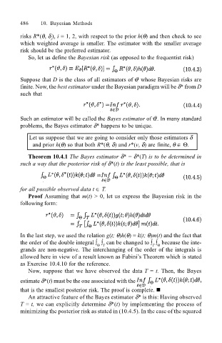
So, let us define the Bayesian risk (as opposed to the frequentist risk)

Suppose that D is the class of all estimators of whose Bayesian risks are
finite. Now, the best estimator under the Bayesian paradigm will be δ* from D
such that

Such an estimator will be called the Bayes estimator of . In many standard
problems, the Bayes estimator δ* happens to be unique.
Let us suppose that we are going to consider only those estimators δ
and prior h(θ) so that both R*(θ, δ) and r*(v, δ) are finite, θ ∈ Θ.

Theorem 10.4.1 The Bayes estimator δ* = δ*(T) is to be determined in
such a way that the posterior risk of δ*(t) is the least possible, that is

for all possible observed data t ∈ T.
Proof Assuming that m(t) > 0, let us express the Bayesian risk in the
following form:

In the last step, we used the relation g(t; θ)h(θ) = k(t; θ)m(t) and the fact that
the order of the double integral ∫ ∫ can be changed to ∫ ∫ because the inte-
T Θ
Θ T
grands are non-negative. The interchanging of the order of the integrals is
allowed here in view of a result known as Fubini’s Theorem which is stated
as Exercise 10.4.10 for the reference.
Now, suppose that we have observed the data T = t. Then, the Bayes
estimate δ*(t) must be the one associated with the
that is the smallest posterior risk. The proof is complete. !
An attractive feature of the Bayes estimator δ* is this: Having observed
T = t, we can explicitly determine δ*(t) by implementing the process of
minimizing the posterior risk as stated in (10.4.5). In the case of the squared