Page 507 - Probability and Statistical Inference

484 10. Bayesian Methods

for 0 < θ < ∞. Now, upon close examination of the rhs of (10.3.6), we realize
that it does resemble a gamma density without its normalizing constant. Hence,
–1
the posterior pdf of v is same as that for the Gamma(t + a, β(nβ + 1) )
distribution. !
For this kind of analysis to go through, the observations X , ..., X n
1
do not necessarily have to be iid to begin with. Look at the
Exercises 10.3.1, 10.3.7, 10.4.2, 10.5.1 and 10.5.8.
Example 10.3.5 Let X , ..., X be iid N(θ, σ ) given that = θ, where v(∈
2
n
1
ℜ) is the unknown population mean and σ(> 0) is assumed known. Consider
the statistic which is minimal sufficient for θ given that v = θ.
Let us suppose that the prior distribution of on the space Θ = ℜ is N(T, δ )
2
where τ (∈ ℜ) and δ (> 0) are known numbers. In order to find the posterior
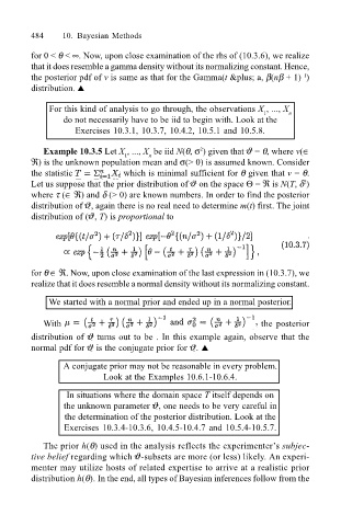
distribution of , again there is no real need to determine m(t) first. The joint
distribution of ( , T) is proportional to

for θ ∈ ℜ. Now, upon close examination of the last expression in (10.3.7), we
realize that it does resemble a normal density without its normalizing constant.
We started with a normal prior and ended up in a normal posterior.

With the posterior

distribution of turns out to be . In this example again, observe that the
normal pdf for is the conjugate prior for . !

A conjugate prior may not be reasonable in every problem.
Look at the Examples 10.6.1-10.6.4.

In situations where the domain space T itself depends on
the unknown parameter , one needs to be very careful in
the determination of the posterior distribution. Look at the
Exercises 10.3.4-10.3.6, 10.4.5-10.4.7 and 10.5.4-10.5.7.
The prior h(θ) used in the analysis reflects the experimenter’s subjec-
tive belief regarding which -subsets are more (or less) likely. An experi-
menter may utilize hosts of related expertise to arrive at a realistic prior
distribution h(θ). In the end, all types of Bayesian inferences follow from the