Page 503 - Probability and Statistical Inference

480 10. Bayesian Methods

Under the Bayesian paradigm, after having the likelihood function and the
prior, the posterior pdf k(θ;t) of v epitomizes how one combines the informa-
tion about obtained from two separate sources, the prior knowledge and
the collected data. The tractability of the final analytical expression of k(θ;t)
largely depends on how easy or difficult it is to obtain the expression of m(t).
In some cases, the marginal distribution of T and the posterior distribution
can be evaluated only numerically.
Example 10.2.1 Let X , ..., X be iid Bernoulli(θ) given that v = θ where v
1
n
is the unknown probability of success, 0 < v < 1. Given v = θ, the statistic
is minimal sufficient for θ, and one has

where T = {0, 1, ..., n}. Now, suppose that the prior distribution of v on the
space Θ = (0, 1) is taken to be Uniform(0, 1), that is h(θ) = I(0 < θ < 1). From
(10.2.2), for t ∈ T, we then obtain the marginal pmf of T as follows:

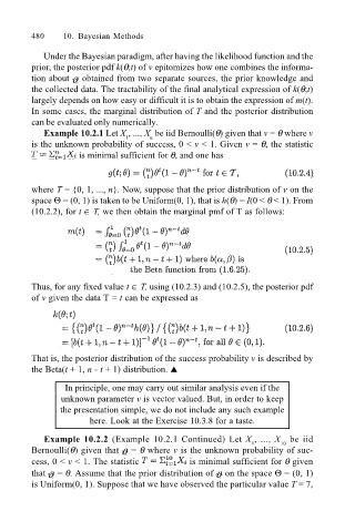
Thus, for any fixed value t ∈ T, using (10.2.3) and (10.2.5), the posterior pdf
of v given the data T = t can be expressed as

That is, the posterior distribution of the success probability v is described by
the Beta(t + 1, n - t + 1) distribution. !
In principle, one may carry out similar analysis even if the
unknown parameter v is vector valued. But, in order to keep
the presentation simple, we do not include any such example
here. Look at the Exercise 10.3.8 for a taste.

Example 10.2.2 (Example 10.2.1 Continued) Let X , ..., X be iid
1
10
Bernoulli(θ) given that = θ where v is the unknown probability of suc-
cess, 0 < v < 1. The statistic is minimal sufficient for θ given
that = θ. Assume that the prior distribution of on the space Θ = (0, 1)
is Uniform(0, 1). Suppose that we have observed the particular value T = 7,