
Page 504 - Probability and Statistical Inference
P. 504
10. Bayesian Methods 481
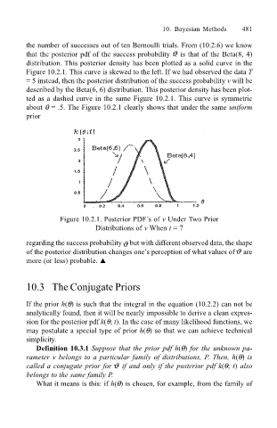
the number of successes out of ten Bernoulli trials. From (10.2.6) we know
that the posterior pdf of the success probability is that of the Beta(8, 4)
distribution. This posterior density has been plotted as a solid curve in the
Figure 10.2.1. This curve is skewed to the left. If we had observed the data T
= 5 instead, then the posterior distribution of the success probability v will be
described by the Beta(6, 6) distribution. This posterior density has been plot-
ted as a dashed curve in the same Figure 10.2.1. This curve is symmetric
about θ = .5. The Figure 10.2.1 clearly shows that under the same uniform
prior
Figure 10.2.1. Posterior PDFs of v Under Two Prior
Distributions of v When t = 7
regarding the success probability but with different observed data, the shape
of the posterior distribution changes ones perception of what values of are
more (or less) probable. !
10.3 The Conjugate Priors
If the prior h(θ) is such that the integral in the equation (10.2.2) can not be
analytically found, then it will be nearly impossible to derive a clean expres-
sion for the posterior pdf k(θ; t). In the case of many likelihood functions, we
may postulate a special type of prior h(θ) so that we can achieve technical
simplicity.
Definition 10.3.1 Suppose that the prior pdf h(θ) for the unknown pa-
rameter v belongs to a particular family of distributions, P. Then, h(θ) is
called a conjugate prior for if and only if the posterior pdf k(θ; t) also
belongs to the same family P.
What it means is this: if h(θ) is chosen, for example, from the family of