Page 132 - Process Equipment and Plant Design Principles and Practices by Subhabrata Ray Gargi Das

5.4 Pinch design analysis 129

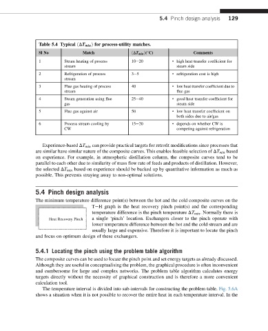
Table 5.4 Typical ðDT min Þ for process-utility matches.
Sl No Match ðDT min Þ( C) Comments

1 Steam heating of process 10e20 · high heat transfer coefficient for
stream steam side
2 Refrigeration of process 3e5 · refrigeration cost is high
stream
3 Flue gas heating of process 40 · low heat transfer coefficient due to
stream flue gas
4 Steam generation using flue 25e40 · good heat transfer coefficient for
gas steam side
5 Flue gas against air 50 · low heat transfer coefficient on
both sides due to air/gas
6 Process stream cooling by 15e20 · depends on whether CW is
CW competing against refrigeration

Experience-based DT min can provide practical targets for retrofit modifications since processes that
are similar have similar nature of the composite curves. This enables feasible selection of DT min based
on experience. For example, in atmospheric distillation column, the composite curves tend to be
parallel to each other due to similarity of mass flow rate of feeds and products of distillation. However,
the selected DT min based on experience should be backed up by quantitative information as much as
possible. This prevents straying away to non-optimal solutions.

5.4 Pinch design analysis
The minimum temperature difference point(s) between the hot and the cold composite curves on the
TeH graph is the heat recovery pinch point(s) and the corresponding
temperature difference is the pinch temperature DT min . Normally there is
Heat Recovery Pinch a single ‘pinch’ location. Exchangers closer to the pinch operate with
lower temperature difference between the hot and the cold stream and are
usually large and expensive. Therefore it is important to locate the pinch
and focus on optimum design of these exchangers.

5.4.1 Locating the pinch using the problem table algorithm

The composite curves can be used to locate the pinch point and set energy targets as already discussed.
Although they are useful in conceptualising the problem, the graphical procedure is often inconvenient
and cumbersome for large and complex networks. The problem table algorithm calculates energy
targets directly without the necessity of graphical construction and is therefore a more convenient
calculation tool.
The temperature interval is divided into sub-intervals for constructing the problem table. Fig. 5.6A
shows a situation when it is not possible to recover the entire heat in each temperature interval. In the