Page 127 - Process Equipment and Plant Design Principles and Practices by Subhabrata Ray Gargi Das

124 Chapter 5 Heat exchanger network analysis

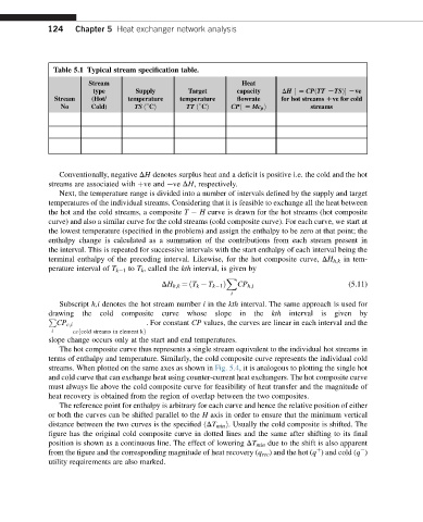
Table 5.1 Typical stream specification table.
Stream Heat
type Supply Target capacity DH ½ [ CPðTT LTSފ Lve
Stream (Hot/ temperature temperature flowrate for hot streams Dve for cold
No Cold) TS ð CÞ TT ð CÞ CPð [ Mc p Þ streams

Conventionally, negative DH denotes surplus heat and a deficit is positive i.e. the cold and the hot
streams are associated with þve and eve DH, respectively.
Next, the temperature range is divided into a number of intervals defined by the supply and target
temperatures of the individual streams. Considering that it is feasible to exchange all the heat between
the hot and the cold streams, a composite T H curve is drawn for the hot streams (hot composite
curve) and also a similar curve for the cold streams (cold composite curve). For each curve, we start at
the lowest temperature (specified in the problem) and assign the enthalpy to be zero at that point; the
enthalpy change is calculated as a summation of the contributions from each stream present in
the interval. This is repeated for successive intervals with the start enthalpy of each interval being the
terminal enthalpy of the preceding interval. Likewise, for the hot composite curve, DH h;k in tem-
perature interval of T k 1 to T k , called the kth interval, is given by
X
CP h;i (5.11)
DH h;k ¼ðT k T k 1 Þ
i
Subscript h,i denotes the hot stream number i in the kth interval. The same approach is used for
drawing the cold composite curve whose slope in the kth interval is given by
P
CP c;i . For constant CP values, the curves are linear in each interval and the
i
cεfcold streams in element kg
slope change occurs only at the start and end temperatures.
The hot composite curve thus represents a single stream equivalent to the individual hot streams in
terms of enthalpy and temperature. Similarly, the cold composite curve represents the individual cold
streams. When plotted on the same axes as shown in Fig. 5.4, it is analogous to plotting the single hot
and cold curve that can exchange heat using counter-current heat exchangers. The hot composite curve
must always lie above the cold composite curve for feasibility of heat transfer and the magnitude of
heat recovery is obtained from the region of overlap between the two composites.
The reference point for enthalpy is arbitrary for each curve and hence the relative position of either
or both the curves can be shifted parallel to the H axis in order to ensure that the minimum vertical
distance between the two curves is the specified ðDT min Þ. Usually the cold composite is shifted. The
figure has the original cold composite curve in dotted lines and the same after shifting to its final
position is shown as a continuous line. The effect of lowering DT min due to the shift is also apparent
from the figure and the corresponding magnitude of heat recovery (q rec ) and the hot (q ) and cold (q )

þ
utility requirements are also marked.