Page 277 - Process Equipment and Plant Design Principles and Practices by Subhabrata Ray Gargi Das

278 Chapter 10 Absorption and stripping

and
" #
1 1
3600 3:205
m L;op ¼ 9400:65 f64 x op þ 18 ð1 x op Þg
ð1 x op Þ
Finding (x i ,y i ) for a typical (x op ,y op ) e
1. Choose a point on the operating line (x op ,y op ), y 2 < y op < y 1
2. Assume f ¼ 1
0
0
3. Calculate m V;op and m L;op from the above expressions. Calculate k x a and k y a from their
expressions at 30 C as discussed above.

4. Draw driving force line through operating point (x op ,y op ), with slope ¼ f (k x a/k y a)
0
0
5. Locate (x i ,y i ) as the intersection of the equilibrium curve and the driving force line drawn.
8 9

ð1 y i Þ 1 y op lnfð1 x i Þ=ð1 x op Þg
< =
Find f calc ¼
ln ð1 y i Þ= 1 y op
:ð1 x i Þ ð1 x op Þ;
6. If fxf calc ,
Then.
0
0
Record (x op ,y op ), (x i ,y i ), m V;op , k x a and k y a.
If the entire range of y op has been covered.
then stop computing, else Go to Step 1.
Else.
Replace f with f calc , Go to Step 3.
End of If statement
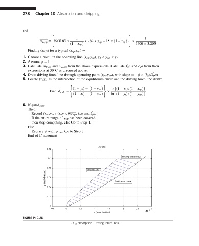
x-y plot
0.12

Driving force line(s)
0.1
0.08 Operating line
y (mole fraction) 0.06 Equilibrium curve

0.04

0.02

0
–0.5 0 0.5 1 1.5 2 2.5 3
–3
×10
x (mole fraction)
FIGURE P10.2C
SO 2 absorptioneDriving force lines.