Page 151 - Process Modelling and Simulation With Finite Element Methods

138 Process Modelling and Simulation with Finite Element Methods

microhydrodynamics simulations of Grammatika and Zimmerman [2], to
consider solving simultaneously with the bulk dynamics. So the coupling is
through simple functional forms learned from simulations of the small scale
dynamics, slaved to the large scale phenomena imposed on it. There are several
drawbacks to the parametric slaving approach, but they are all summed up
by “oversimplification”. Fortunately, such models can be verified by
experimentation that the physical systems can be well treated by the two scale
approach. Traditional turbulence models are all heavily reliant on multiple scale
modeling by parametrization. Since the multiple scale modeling techniques are
specialized, perhaps extended multiphysics is not such a useful feature after all.
To take advantage of it for complex modeling may require high performance
computing.
Only belatedly did it occur to me that chemical engineering is awash with
applications for extended multiphysics. First, let’s give an operational definition
for extended multiphysics in the FEMLAB sense: a model is categorized as
extended multiphysics if it requires description of field variables in two or more
logically disjoint domains. They are not likely to be physically disjoint domains
since the physics must be coupled in some respect to warrant solving the
problems in each domain jointly. FEMLAB allows the user to use several
different geometries/application mode pairs in building up an extended
multiphysics model.
So why is it that chemical engineering is awash with extended multiphysics?
Look no further than your nearest flowsheet, say Figure 4.1.

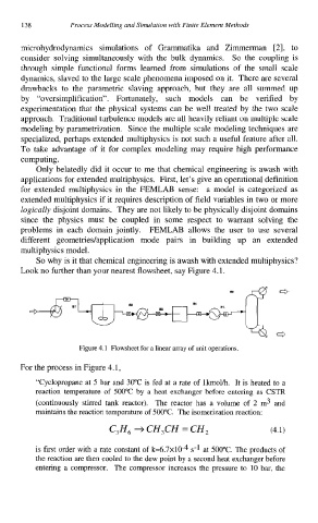
Figure 4.1 Flowsheet for a linear array of unit operations.

For the process in Figure 4.1,
“Cyclopropane at 5 bar and 30°C is fed at a rate of lkmolh. It is heated to a
reaction temperature of 500°C by a heat exchanger before entering as CSTR
(continuously stirred tank reactor). The reactor has a volume of 2 m3 and
maintains the reaction temperature of 500°C. The isomerization reaction:
C,H, + CH,CH = CH, (4.1)

is first order with a rate constant of k=6.7~10-~ s-l at 500°C. The products of
the reaction are then cooled to the dew point by a second heat exchanger before
entering a compressor. The compressor increases the pressure to 10 bar, the