Page 154 - Process Modelling and Simulation With Finite Element Methods

Extended Multiphysics 141

The fluxes j take the traditional mass transfer coefficient form
ju = ~~(u-ii)

jv = IC,,(V--V”) (4.4)

j, = K,(w-w)
At steady state, these fluxes are all equal and thus give two constraints on the
bulk variables u,v,w and on the disperse phase concentrations u” , v“, I?. The
sixth constraint is on the surface reaction, which is presumed to be in equilibrium
(fast reaction kinetics and nearly irreversible):
iiv” - KI? = 0 (4.5)
The boundary conditions will be taken as fixed concentrations of u and v at the
inlet, no w, and outlet conditions with convection much greater than diffusion.
For simplicity, since there are so many parameters, we will test just kinetic
asymmetry of the mass transfer parameters and fix unit diffusivities D,=D,= 1,
mobile product k,=100 and D,=0.001, one of the reactants to have unit mass
transfer coefficient k,=l, and this leaves free parameters as the velocity U and
mass transfer coefficient of the most resistive reactant, k,, reactor length L, and
equilibrium constant K. Since industrial interest lies in reactions that favor the
products, we shall take K=10-5 as a nearly irreversible reaction. Initially, let’s
consider a reactor of length L=5, velocity U=0.5, and mass transfer asymmetry
with k,=0.2. The inlet conditions will be uO=1 and v0=0.4.
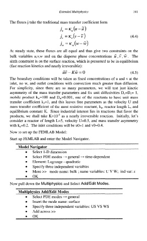
Now to set up the FEMLAB Model:
Start up FEMLAB and enter the Model Navigator.

Model Navigator
Select 1-D dimension
Select PDE modes + general - time-dependent
Element: Lagrange - quadratic
Specify three independent variables
More >> mode name: bulk ; name variables: U V W; ind var: z
0 OK
Now pull down the Multiphysics and Select Add/Edit Modes.
Multiphysics Add/Edit Modes
0 Select PDE modes - general
Insert the mode name: surface
Specify three independent variables: US VS WS
0 Add across >>
0 OK