Page 146 - Process Modelling and Simulation With Finite Element Methods

Multiphysics 133

On to the MATLAB m-file function for the u-velocity

function u=pelletu(x,y)
%PELLETU Interpolates u from the FEM solution for the pellet
% U = PELLETU(X,Y)
% is interpolated on the rectangle [0,0.0021 x [0.0061
load pellet-flow.mat xx yy uu w
% Interpolate from rectangular grid to unstructured point.
u=interp2 (xx,
yy, uu, x, y) ;
Similarly for the v-velocity

function v=pelletv (x,y)
%PELLETV Interpolates u from the FEM solution for the pellet
% V = PELLETV(X,Y)
% is interpolated on the rectangle [0,0.0021 x [0.0061
load pellet-flow.mat xx yy uu w;
% Interpolate from rectangular grid to unstructured point.
v=interp2 (xx,yy,w,x,y)
;
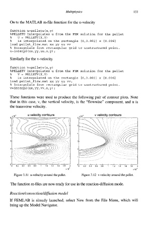
These functions were used to produce the following pair of contour plots. Note
that in this case, v, the vertical velocity, is the "flowwise" component, and u is
the transverse velocity.

v velocitv
contours
4,' v velocity contours

I I
'0 02 04 06 08 1 12 14 16 10 2 Od 0'2 0'4 06 0'8 1'2 1'4 16 1'8 i
10' x 10'
Figure 3.1 1 u-velocity around the pellet. Figure 3.12 v-velocity around the pellet.

The function m-files are now ready for use in the reaction-diffusion mode.
Reactiodconvectioddifision model

If FEMLAB is already launched, select New from the File Menu, which will
bring up the Model Navigator.