Page 145 - Process Modelling and Simulation With Finite Element Methods

132 Process Modelling and Simulation with Finite Element Methods

Max 0252
Contour: velocity field (U-ns)
0 2399
0 2279
0 2159
0 2039
0 1919
0 1799
0 1679
0 1559
0 1439
0 1319
0 1199
0 1079
0 096
o 084
0 072
0 06
0 048
0 036
0 024
0 012
-4 -3 -2 -1 0 0.9 2 3 4 5 6 7
Min 0
10'~
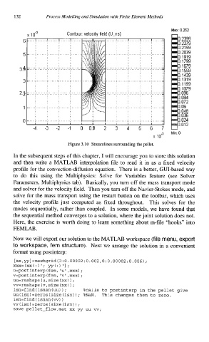
Figure 3.10 Streamlines surrounding the pellet.
In the subsequent steps of this chapter, I will encourage you to store this solution
and then write a MATLAB interpolation file to read it in as a fixed velocity
profile for the convection-diffusion equation. There is a better, GUI-based way
to do this using the Multiphysics: Solve for Variables feature (see Solver
Parameters, Multiphysics tab). Basically, you turn off the mass transport mode
and solver for the velocity field. Then you turn off the Navier-Stokes mode, and
solve for the mass transport using the restart button on the toolbar, which uses
the velocity profile just computed as fixed throughout. This solves for the
modes sequentially, rather than coupled. In some models, we have found that
the sequential method converges to a solution, where the joint solution does not.
Here, the exercise is worth doing to learn something about m-file "hooks" into
FEMLAB .

Now we will export our solution to the MATLAB workspace (file menu, export
to workspace, fem structure). Next we arrange the solution in a convenient
format using postinterp:
[xx,yyl =meshgrid(O: 0.00002: 0.002,O: 0.00002: 0.006) ;
xxx= [xx( :) ' ; yy( :) 'I ;
u=postinterp(fem,'u',xxx);
v=postinterp(fem,'v',xxx);
uu=reshape (u, size (xx) ;
)
w=reshape (v, size (xx) ;
)
)
isn=f ind (isnan (uu) ; %calls to postinterp in the pellet give
uu(isn) =zeros (size (isn) ; %NaN. This changes them to zero.
isn=find(isnan(w) )
)
w(isn) =zeros (size (isn) ;
save pellet-flow.mat xx yy uu w;