Page 143 - Process Modelling and Simulation With Finite Element Methods

130 Process Modelling and Simulation with Finite Element Methods

this does not change the momentum transport. So rather than computing both
momentum transport and mass transport simultaneously, we can compute them
sequentially. Why? Primarily because of the computing efficiency. If one requires
several solutions over a range of mass transportheaction parameters, but with the
same flow field, then computing the flow field only once and importing the velocity
field is the most computationally efficient method (or should be, if coded
efficiently). Secondly, whatever platform you use to compute on is probably
memory limited if you want to refine the mesh. For instance, because we computed
the streamfunction explicitly in the buoyant convection example earlier, it was not
possible to refine the mesh further without running out of system memory on a 1Gb
RAM linux PC workstation. The final reason is that it illustrates further handles
into the FEMLAB GUI through MATLAB programming, which is one of the
reasons to read this text.
We visited the Incompressible Navier-Stokes (2-D) mode in $3.1, and in fact
if we add a reaction source term to (3.1) and call concentration T rather than c, then
those equations describe the model perfectly.
Launch FEMLAB and in the Model Navigator, select the Multiphysics tab.

Model Navigator
Select 2-D dimension
Select Physics modes+Incompressible Navier-Stokes >>
OK

We will now follow the recipe on [9], p. 2-78ff to construct the configuration
and Navier-Stokes solution around the pellet. Set up the axis and grid as follows
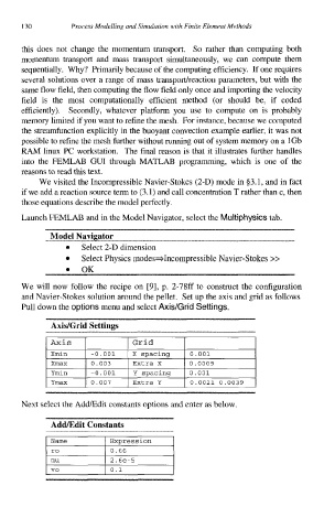
Pull down the options menu and select Axis/Grid Settings.

AxisIGrid Settings
Axis Grid
Xmin -0.001 X spacing 0.001
Xmax 0.003 Extra X 0.0009
Ymin -0.001 Y suacinu 0.001
I I I I
I Ymax I 0.007 I Extra Y I 0.0021 0.0039 I
Next select the AddEdit constants options and enter as below.

Add/Edit Constants

Expression
2. be-5
vo