Page 141 - Process Modelling and Simulation With Finite Element Methods

128 Process Modelling and Simulation with Finite Element Methods

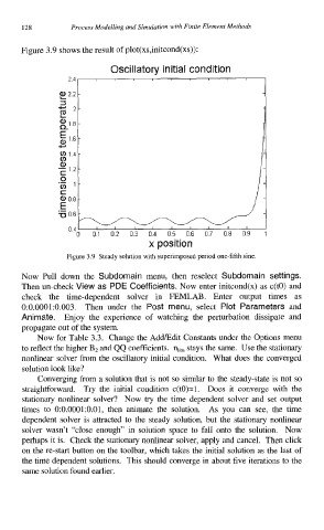
Figure 3.9 shows the result of plot(xs,initcond(xs)):
Oscillatory initial condition
24

x position
Figure 3.9 Steady solution with superimposed period one-fifth sine

Now Pull down the Subdomain menu, then reselect Subdomain settings.
Then un-check View as PDE Coefficients. Now enter initcond(x) as c(t0) and
check the time-dependent solver in FEMLAB. Enter output times as
0:0.0001:0.003. Then under the Post menu, select Plot Parameters and
Animate. Enjoy the experience of watching the perturbation dissipate and
propagate out of the system.
Now for Table 3.3. Change the AddEdit Constants under the Options menu
to reflect the higher B2 and QQ coefficients. nlim stays the same. Use the stationary
nonlinear solver from the oscillatory initial condition. What does the converged
solution look like?
Converging from a solution that is not so similar to the steady-state is not so
straightforward. Try the initial condition c(tO)=l. Does it converge with the
stationary nonlinear solver? Now try the time dependent solver and set output
times to 0:0.0001:0.01, then animate the solution. As you can see, the time
dependent solver is attracted to the steady solution, but the stationary nonlinear
solver wasn’t “close enough” in solution space to fall onto the solution. Now
perhaps it is. Check the stationary nonlinear solver, apply and cancel. Then click
on the re-start button on the toolbar, which takes the initial solution as the last of
the time dependent solutions. This should converge in about five iterations to the
same solution found earlier.