Page 140 - Process Modelling and Simulation With Finite Element Methods

Multiphysics 127

Now for the Solver. Pull down the Solver Menu and select Parameters.
Check the Stationary Nonlinear solver box, apply, and click on the Solve button.
It takes FEMLAB 25 iterations to get there (this is a highly nonlinear problem),
but it converges to 10.' accuracy eventually. 1 played around with several
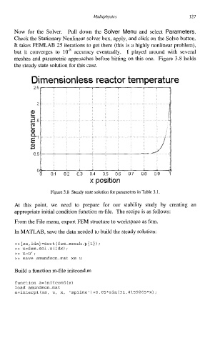
meshes and parametric approaches before hitting on this one. Figure 3.8 holds
the steady state solution for this case.

Dimensionless reactor temperature

x position
Figure 3.8 Steady state solution for parameters in Table 3.1

At this point, we need to prepare for our stability study by creating an
appropriate initial condition function m-file. The recipe is as follows:
From the File menu, export FEM structure to workspace as fem.
In MATLAB, save the data needed to build the steady solution:

>>[x~,idxl=sort(fem.xmesh.p{l})
;
>> u=fern.sol.u(idx) ;
>> u=u';
>> save arnundson.mat xs u
Build a function m-file initc0nd.m

function a=initcond (x)
load amundson.mat
a=interpl(xs, u, x, 'spline')+O.OS*sin(31.4159265*~);