Page 195 - Process Modelling and Simulation With Finite Element Methods

182 Process Modelling and Simulation with Finite Element Methods

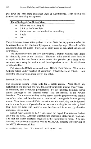
Pull down the Point menu and select View as Coefficients. Then select Point
Settings and the dialog box appears.

Select any vertex (say 4)
Click on the Weak Tab
Under constraint replace the first zero with -p
Apply

The point datum is now set to p=O on vertex 4. Note that any pressure value can
be entered here as the constraint by replacing a zero by PO-p. The order of the
constraints does not matter. There are as many zeros as dependent variables in
your model.
The second reason for the slow convergence is that the velocity field should
be identically zero as the solution. However, noise around zero interacts
strangely with the new feature of the solver that permits the scaling of the
estimated error using the nonlinear and time-dependent solvers. So this feature
must be disabled.
Pull down the Solver menu and select Solver Parameters. Click on the
Settings button under “Scaling of variables.” Check the None option. Now
select the Stationary Nonlinear solver, and solve.

Internal Gravity Waves
The automatic scaling setting fails for a subtle reason. With Ra<O, any
perturbation or numerical error excites a small amplitude internal gravity wave -
an inherently time dependent phenomenon. So the stationary nonlinear solver
cannot converge to the “internal waves” that are inherent in the Newton
iterations. The automatic scaling setting senses that the proper velocity scale is
that of the noise, and therefore tries to resolve and converge the internal gravity
waves. Since these are small if the numerical error is small, they can be ignored,
which is what happens if you disable the automatic scaling for the velocity field.
That there are wave like solutions can be discerned from an eigenfunction
analysis of the solution.
Export your solution to MATLAB using the export fem structure feature
under the file menu. Although eigenfunction analysis is supported in FEMLAB,
it is only for linear problems specified in the eigenfunction mode. You can,
however, use the built-in analysis tools in MATLAB. Execute the following on
the MATLAB command line:
>> sol2=femeig(fem, ‘U’, fem.sol.u,’Eigpari,20);