Page 200 - Process Modelling and Simulation With Finite Element Methods

Simulation and Nonlinear Dynamics 187

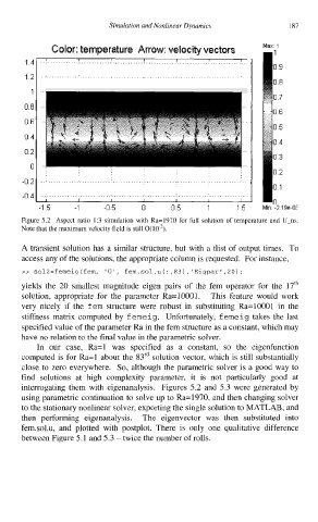
Color: temperature Arrow: velocity vectors Max 1
1
1.4 ....................................................................................
I
09
1.2 ....................................................................................
08
1
07
0.8
06
0.6
05
0.4
04
0.2
03
0
02
-0.2 ...................................................................................
01
-0.4 ....................................................................................
I I I I I I I 0
-1.5 -1 -0 5 0 0.5 1 1.5 Min -2 19e-0:
Figure 5.2 Aspect ratio 1.3 simulation with Ra=1970 for full solution of temperature and U-ns.
Note that the maximum velocity field is still 0(10-*).

A transient solution has a similar structure, but with a tlist of output times. To
access any of the solutions, the appropriate column is requested. For instance,

>> sol2=femeig(fem, 'U', fem.sol.u(:,83),'Eigpar',20);
yields the 20 smallest magnitude eigen pairs of the fem operator for the 17'h
solution, appropriate for the parameter Ra=10001. This feature would work
very nicely if the fem structure were robust in substituting Ra=10001 in the
stiffness matrix computed by f emeig. Unfortunately, f emeig takes the last
specified value of the parameter Ra in the fern structure as a constant, which may
have no relation to the final value in the parametric solver.
In our case, Ra=l was specified as a constant, so the eigenfunction
computed is for Ra=l about the 83'd solution vector, which is still substantially
close to zero everywhere. So, although the parametric solver is a good way to
find solutions at high complexity parameter, it is not particularly good at
interrogating them with eigenanalysis. Figures 5.2 and 5.3 were generated by
using parametric continuation to solve up to Ra=1970, and then changing solver
to the stationary nonlinear solver, exporting the single solution to MATLAB, and
then performing eigenanalysis. The eigenvector was then substituted into
fem.sol.u, and plotted with postplot. There is only one qualitative difference
between Figure 5.1 and 5.3 - twice the number of rolls.