Page 199 - Process Modelling and Simulation With Finite Element Methods

186 Process Modelling and Simulation with Finite Element Methods

one wave per two units length), a domain of length 3 is sufficiently long to
encompass one period of the unstable mode at supercriticality.
Our solution strategy is to compute the Ra=l solution first using the linear
solver, and then use the Parametric Solver to continue to high Rayleigh number,
finding the unstable mode visually from plots of the velocity field. At first I
thought that this does not yield a visually unstable flow, even up to Ra=10000
(see Figure 5.2). Why not? u=v=p=T=O is a perfectly acceptable numerical
solution, and the model finds solutions with small dimensionless convective
flows, with velocity magnitudes of 0(10-*), for all values of the Rayleigh
number attempted. Professor Bruce Finlayson and chemical engineering student
Michael Johnson (private communication) pointed out that since the Nusselt
number scales with the Rayleigh number, these are actually giving rise to
appreciable convective heat flux. However, there is no specific threshold of Ra
which is apparently an abrupt change in Nusselt number. To find the Rac,
something else must be tried. The obvious strategy is to use transient integration
to determine if, after a sufficiently long time, random small magnitude initial
conditions have grown expontially large as in (5.4). The problem with this is
that FEMLAB’s Parametric Solver only applies to stationary models. The other
solution is to compute the eigenanalysis for the system at each value of Ra in a
parametric continuation of Ra to high Rayleigh numbers. We will do this two
ways: one in the GUI, exporting solutions to the MATLAB workspace; the other
in a MATLAB m-file with continuation implemented in a MATLAB loop
structure. The results are edifying about the nature of the f emeig command in
the FEMLAB programming library.

GUI Methodology
Figure 5.2 was generated from solving the Benard problem using parametric
continuation in the GUI. The linear solver for the Ra=l problem was used,
which is well conditioned. Parametric Solver was used to continue to high
Rayleigh number. For eigenanalysis, we export our solution to MATLAB using
the export fem structure feature under the file menu. The data structure for a
parametric solution is different than for a single, stationary solution. For
instance, for the case of a parametric solution [1801:100:10001], fem.sol is an
array with three elements: u (the solution), plist (parameter list), and pname (the
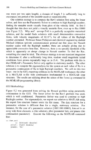
continuation parameter). Execute the following on the MATLAB command
line:
>> fem.so1
u: [6966x83 double]
plist: [1x83 double]
pname: ’Ra’