Page 201 - Process Modelling and Simulation With Finite Element Methods

188 Process Modelling and Simulation with Finite Element Methods
Ma: i 0105 Max 000356
3

o:i , , , , , , 4

,

-1 5 -1 -0 5 0 05 1 Mln 0 Min -000355
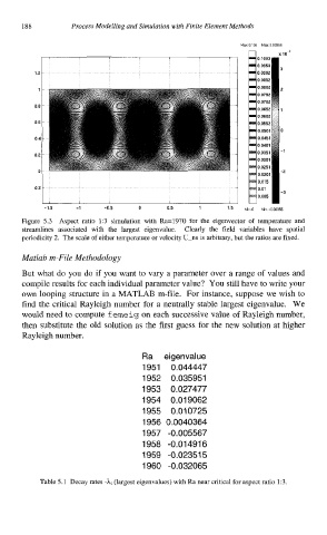
Figure 5.3 Aspect ratio 1:3 simulation with Ra=1970 for the eigenvector of temperature and
streamlines associated with the largest eigenvalue. Clearly the field variables have spatial
periodicity 2. The scale of either temperature or velocity U-ns is arbitrary, but the ratios are fixed.
Matlab m-File Methodology

But what do you do if you want to vary a parameter over a range of values and
compile results for each individual parameter value? You still have to write your
own looping structure in a MATLAB m-file. For instance, suppose we wish to
find the critical Rayleigh number for a neutrally stable largest eigenvalue. We
would need to compute f emeig on each successive value of Rayleigh number,
then substitute the old solution as the first guess for the new solution at higher
Rayleigh number.
Ra eigenvalue
1951 0.044447
1952 0.035951
1953 0.027477
1954 0.01 9062
1955 0.01 0725
1956 0.0040364
1957 -0.005567
1958 -0.01 491 6
1959 -0.02351 5
1960 -0.032065
Table 5.1 Decay rates -hi (largest eigenvalues) with Ra near critical for aspect ratio 1:3.