Page 196 - Process Modelling and Simulation With Finite Element Methods

Simulation and Nonlinear Dynamics 183

The arguments are described in the Reference Manual, however, it should be
clear that fem is a fem structure, ‘U’ specifies that the next argument is a solution
vector; fem.so1.u is that solution found for Ra=-1; ‘Eigpar’ is a flag that says the
next argument describes the requested eigenvalue solver parameters (in this case
the smallest 20 eigenvalues in magnitude).
This generates a structure so12 with substructures sol2.u and sol2.lambda.
You probably find that sol2.lambda has twenty elements, and that sol2.u is a
matrix with twenty columns and a huge number of rows. Each column is an
eigenvector associated with the same numbered eigenvalue. Femeig uses
iterative sparse methods for generating eigenvalue/eigenvector pairs. By default,
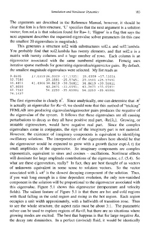
the smallest magnitude eigenvalues were selected. My list reads as

9.8695 17.0399 26.0309 -17.1321i 26.0309 +17.1321i
32.7180 29.1581 -25.5745i 29.1581 +25.5745i
39.4811 41.4966 34.8619 -30.5681i 34.8619 +30.5681i
47.8093 43.2471 -33.6591i 43.2471 +33.6591i
60.7142 54.2250 -35.6500i 54.2250 +35.6500i
74.1437
The first eigenvalue is clearly n2. Since analytically, one can determine that -n2
is actually an eigenvalue for Ra=O, we should note that this method of “tricking”
FEMLAB into producing eigenvalue/eigenvector pairs produces the negative of
the eigenvalue of the system. It follows that these eigenvalues are all causing
perturbations to decay as they all have positive real part, -Re{ A,). Growing, or
unstable eigenvectors, would have negative real part. Since the complex
eigenvalues come in conjugates, the sign of the imaginary part is not material.
However, the existence of imaginary components is equivalent to identifying
oscillatory solutions. The interpretation of the eigenvalues here should be that
the eigenvector would be expected to grow with a growth factor exp(-h t) for
small amplitudes of the eigenvector. So imaginary components are complex
exponentials, equivalent to sines and cosines - oscillations. Nonlinear effects
will dominate for large amplitude contributions of the eigenvector, c.f. (5.4). So
what are these eigenvectors, really? In fact, they are best thought of as vectors
of unknowns equivalent in some sense to solution vectors. So the vector
associated with h =n2 is the slowest decaying component of the solution. Thus,
if you wait long enough in a time dependent evolution, the only non-vanished
component in the solution will be proportional to the eigenvector associated with
this eigenvalue. Figure 5.1 shows this eigenvector (temperature and velocity
fields). The salient feature of Figure 5.1 is that there are hot and cold regions
with fluid falling in the cold region and rising in the hot region. Each region
occupies a unit width approximately, with a halfwidth of transition zone. Thus
to see the whole structure, the aspect ratio must be about 3: 1. The parametric
solver can be used to explore regions of Ra<O, but there are no situations where
growing modes are excited. The best that happens is that for large negative Ra,
the decay rate diminishes. In a perfect (inviscid) fluid, it would be identically