Page 245 - Process Modelling and Simulation With Finite Element Methods

232 Process Modelling and Simulation with Finite Element Methods

Now
the
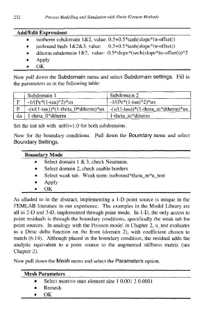
Subdomain 1 Subdomain 2
r - l/(Pe*( 1 -tau)"2)*ux - 1 /( Pe*( 1 -tau)"2) *ux
F -(d( 1-tau))*( 1-theta-O*dtherm)*ux -(d( 1-tau))*( 1 -theta-m*dtherm)*ux
da l-theta-O*dtherm 1 -theta-m*dtherm
Set

Now
Boundary

Boundary Mode
Select domain 1 & 3, check Neumann.
0
Select domain 2, check enable borders
Select weak tab. Weak term: isobound*theta-m*u-test
Apply
OK
0
As alluded to in the abstract, implementing a 1-D point source is unique in the
FEMLAB literature in our experience. The examples in the Model Library are
all in 2-D and 3-D, implemented through point mode. In 1-D, the only access to
point residuals is through the boundary conditions, specifically the weak tab for
point sources. In analogy with the Poisson model in Chapter 2, u-test evaluates
as a Dirac delta function on the front (domain 2), with coefficient chosen to
match (6.14). Although placed in the boundary condition, the residual adds the
analytic equivalent to a point source to the augmented stiffness matrix (see
Chapter 2).
Now pull down the Mesh menu and select the Parameters option.

Mesh Parameters
Select more>> max element size 1 0.001 2 0.0001
Remesh
0 OK