Page 246 - Process Modelling and Simulation With Finite Element Methods

Geometric Continuation 233

There should be 1245 elements.

Now enter solver mode and select solver parameters. Select weak form. Set
time stepping 0:0.001:0.01. Now solve. Then save a model m-file as the single
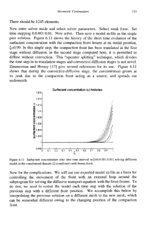
pass solution. Figure 6.11 shows the history of the short time evolution of the
surfactant concentration with the compaction front frozen at its initial position,
5=0.99. In this single step, the compaction front has been translated in the first
stage without diffusion, in the second stage computed here, it is permitted to
diffuse without convection. This “operator splitting” technique, which divides
the time step in to translation stages and convective-diffusion stages is not novel.
Zimmerman and Homsy [17] give several references for its use. Figure 6.11
shows that during the convective-diffusive stage, the concentration grows at
its peak due to the compaction front acting as a source, and spreads out
underneath.

Surfactant concentration (u) histories
I
1.0141

oggsl ’ ’ ’ ’ ’ ’ ’ ’ ’ ’
n 01 02 03 06 07 08 09 1
O4 GO5
Figure 6.11 Surfactant concentration after first time interval tE [0.0:0.001:0.01] solving diffusion
model in the transformed domain (6-coordinate) with frozen front.
Now for the complications. We will use our exported model m-file as a basis for
controlling the movement of the front with an external loop around the
subprogram for solving the diffusive transport equation with the front frozen. To
do this, we need to restart the model each time step with the solution of the
previous step with a different front position. We accomplish this below by
interpolating the previous solution on a different mesh to the new mesh, which
can be somewhat different owing to the changing position of the compaction
front.