Page 26 - Process Modelling and Simulation With Finite Element Methods

Introduction to FEMLAB 13
analyzed geometries. Although the geometry specification can be done
graphically in Draw mode, it can also be done through MATLAB functions, a
power that is exploited in Chapter six on geometrical continuation.
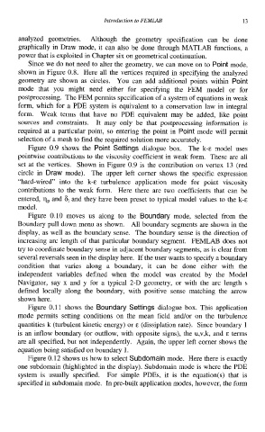
Since we do not need to alter the geometry, we can move on to Point mode,
shown in Figure 0.8. Here all the vertices required in specifying the analyzed
geometry are shown as circles. You can add additional points within Point
mode that you might need either for specifying the FEM model or for
postprocessing. The FEM permits specification of a system of equations in weak
form, which for a PDE system is equivalent to a conservation law in integral
form. Weak terms that have no PDE equivalent may be added, like point
sources and constraints. It may only be that postprocessing information is
required at a particular point, so entering the point in Point mode will permit
selection of a mesh to find the required solution more accurately.
Figure 0.9 shows the Point Settings dialogue box. The k-& model uses
pointwise contributions to the viscosity coefficient in weak form. These are all
set at the vertices. Shown in Figure 0.9 is the contribution on vertex 13 (red
circle in Draw mode). The upper left comer shows the specific expression
"hard-wired" into the k-E turbulence application mode for point viscosity
contributions to the weak form. Here there are two coefficients that can be
entered, qp and z1 and they have been preset to typical model values to the k-E
model.
Figure 0.10 moves us along to the Boundary mode, selected from the
Boundary pull down menu as shown. All boundary segments are shown in the
display, as well as the boundary sense. The boundary sense is the direction of
increasing arc length of that particular boundary segment. FEMLAB does not
try to coordinate boundary sense in adjacent boundary segments, as is clear from
several reversals seen in the display here. If the user wants to specify a boundary
condition that varies along a boundary, it can be done either with the
independent variables defined when the model was created by the Model
Navigator, say x and y for a typical 2-D geometry, or with the arc length s
defined locally along the boundary, with positive sense matching the arrow
shown here.
Figure 0.11 shows the Boundary Settings dialogue box. This application
mode permits setting conditions on the mean field and/or on the turbulence
quantities k (turbulent kinetic energy) or E (dissiplation rate). Since boundary 1
is an inflow boundary (or outflow, with opposite signs), the u,v,k, and E terms
are all specified, but not independently. Again, the upper left corner shows the
equation being satisfied on boundary 1.
Figure 0.12 shows us how to select Subdomain mode. Here there is exactly
one subdomain (highlighted in the display). Subdomain mode is where the PDE
system is usually specified. For simple PDEs, it is the equation(s) that is
specified in subdomain mode. In pre-built application modes, however, the form