Page 27 - Process Modelling and Simulation With Finite Element Methods

14 Process Modelling and Simulation with Finite Element Methods

of the equations is “hard-wired” in, and only the coefficients are specified in
subdomain mode.
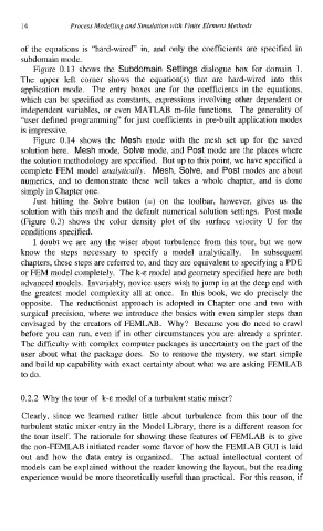
Figure 0.13 shows the Subdomain Settings dialogue box for domain 1.
The upper left comer shows the equation(s) that are hard-wired into this
application mode. The entry boxes are for the coefficients in the equations,
which can be specified as constants, expressions involving other dependent or
independent variables, or even MATLAB m-file functions. The generality of
“user defined programming” for just coefficients in pre-built application modes
is impressive.
Figure 0.14 shows the Mesh mode with the mesh set up for the saved
solution here. Mesh mode, Solve mode, and Post mode are the places where
the solution methodology are specified. But up to this point, we have specified a
complete FEM model analytically. Mesh, Solve, and Post modes are about
numerics, and to demonstrate these well takes a whole chapter, and is done
simply in Chapter one.
Just hitting the Solve button (=) on the toolbar, however, gives us the
solution with this mesh and the default numerical solution settings. Post mode
(Figure 0.3) shows the color density plot of the surface velocity U for the
conditions specified.
I doubt we are any the wiser about turbulence from this tour, but we now
know the steps necessary to specify a model analytically. In subsequent
chapters, these steps are referred to, and they are equivalent to specifying a PDE
or FEM model completely. The k-E model and geometry specified here are both
advanced models. Invariably, novice users wish to jump in at the deep end with
the greatest model complexity all at once. In this book, we do precisely the
opposite. The reductionist approach is adopted in Chapter one and two with
surgical precision, where we introduce the basics with even simpler steps than
envisaged by the creators of FEMLAB. Why? Because you do need to crawl
before you can run, even if in other circumstances you are already a sprinter.
The difficulty with complex computer packages is uncertainty on the part of the
user about what the package does. So to remove the mystery, we start simple
and build up capability with exact certainty about what we are asking FEMLAB
to do.

0.2.2 Why the tour of k-E model of a turbulent static mixer?
Clearly, since we learned rather little about turbulence from this tour of the
turbulent static mixer entry in the Model Library, there is a different reason for
the tour itself. The rationale for showing these features of FEMLAB is to give
the non-FEMLAB initiated reader some flavor of how the FEMLAB GUI is laid
out and how the data entry is organized. The actual intellectual content of
models can be explained without the reader knowing the layout, but the reading
experience would be more theoretically useful than practical. For this reason, if