Page 31 - Process Modelling and Simulation With Finite Element Methods

18 Process Modelling and Simulation with Finite Element Methods

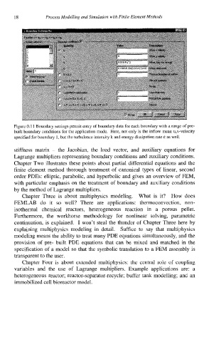
Figure 0.1 1 Boundary settings permit entry of boundary data for each boundary with a range of pre-
built boundary conditions for the application mode. Here, not only is the inflow mean u,v-velocity
specified for boundary 1, but the turbulence intensity k and energy dissipation rate E as well.

stiffness matrix - the Jacobian, the load vector, and auxiliary equations for
Lagrange multipliers representing boundary conditions and auxiliary conditions.
Chapter Two illustrates these points about partial differential equations and the
finite element method thorough treatment of canonical types of linear, second
order PDEs: elliptic, parabolic, and hyperbolic and gives an overview of FEM,
with particular emphasis on the treatment of boundary and auxiliary conditions
by the method of Lagrange multipliers.
Chapter Three is about multiphysics modeling. What is it? How does
FEMLAB do it so well? There are applications: thermoconvection, non-
isothermal chemical reactors, heterogeneous reaction in a porous pellet.
Furthermore, the workhorse methodology for nonlinear solving, parametric
continuation, is explained. I won’t steal the thunder of Chapter Three here by
explaining multiphysics modeling in detail. Suffice to say that multiphysics
modeling means the ability to treat many PDE equations simultaneously, and the
provision of pre- built PDE equations that can be mixed and matched in the
specification of a model so that the symbolic translation to a FEM assembly is
transparent to the user.
Chapter Four is about extended multiphysics: the central role of coupling
variables and the use of Lagrange multipliers. Example applications are: a
heterogeneous reactor; reactor-separator-recycle; buffer tank modelling; and an
immobilized cell bioreactor model.