Page 315 - Process Modelling and Simulation With Finite Element Methods

302 Process Modelling and Simulation with Finite Element Methods
mx I52
T,mp = 0 1
14
12
1
06
04
02
0
02
04
06
0681
MBX 109 0 738
1
06
04
06 4
02
0
0
02
3
05 04
M“ 0597 0 1 M,” 047s
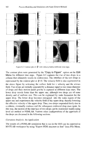
Figure 8.2 Contour plot of with velocity field at different time steps.

The contour plots were generated by the “Copy to Figure” option on the Edit
Menu for different time steps. Figure 8.2 captures the rise of two drops in a
column that ultimately results in coalescence. The interface of the two drops is
represented by the contour plot at @ =O. The velocity field is also represented in
the above figure by activating the surface field for v velocity and the arrows
field. Two drops are initially separated by a distance equal to two times diameter
of drops and their motion under gravity is captured at different time steps. The
lower drop travels faster than the upper one, although two drops are of same
density and of uniform size. This can be explained by wake formation for the
upper drop. The lower drop becomes entrapped into the wake region of the
upper one and experiences the velocity field of the upper drop, thereby lowering
the effective velocity of the upper drop. Thus, two drops suspended freely rise in
a column, eventually coalesce and the subsequent coalesced drop rises again. In
this way, the motion of the interface of two drops can be monitored readily using
level set method in FEMLAB. Various other configurations of the approach of
the drops are discussed in the following sections.

Curvature Analysis: An Application

The results of a FEMLAB simulation that is run in the GUI can be exported to
MATLAB workspace by using “Export FEM structure as fem” from File Menu.