Page 316 - Process Modelling and Simulation With Finite Element Methods

Modeling of Multi-Phase Flow Using the kvel Set Method 303

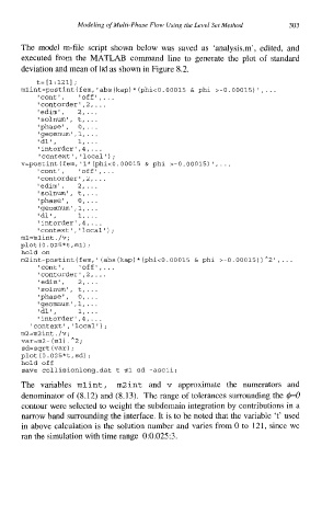
The model m-file script shown below was saved as 'analysis.m', edited, and
executed from the MATLAB command line to generate the plot of standard
deviation and mean of Id as shown in Figure 8.2.
t= [l: 1211 ;
mlint=postint (fern, labs (kap) * (phi<O. 00015 & phi >-0.00015) I , . . .
'cont', 'off', ...
I contorder' ,2, . . .
'edim', 2,. . .
'solnum' t, . . .
,
'phase', 0,. . .
'geomnurn' ,1, . .
.
'dl' , 1, ...
'intorder',4, ...
'
' context ' , I local ) ;
v=postint(fem,'1*(phic0.00015 phi >-0.00015) I, _ ..
&
'cont', 'off', ...
'contorder',2, ...
'edim', 2,. . .
'solnum', t, ...
'phase', 0,. .
.
.
'geomnurn',l,. .
'dl', 1, ...
'intorder',4, ...
'context','local');
ml=mlint./v;
plot (0.025*t,ml)
;
hold on
rn2int=postint(fern,' (abs(kap)*(phi<0.00015 & phi >-0.00015))A2',...
'cont', 'off', ...
'contorder',2, ...
.
'edim', 2,. .
'solnum', t,. . .
'phase', 0, ...
.
'geomnurn' ,1, . .
'dl', 1, ...
'intorder',4, ...
'context','local')
;
m2=m2int./v;
var=m2- (ml) .*2;
sd=sqrt (var) ;
plot(O.OZS*t,sd) ;
hold off
save collisionlong.dat t ml sd -ascii;
The variables mlint , m2int and v approximate the numerators and
denominator of (8.12) and (8.13). The range of tolerances surrounding the $=o
contour were selected to weight the subdomain integration by contributions in a
narrow band surrounding the interface. It is to be noted that the variable 't' used
in above calculation is the solution number and varies from 0 to 121, since we
ran the simulation with time range 0:0.025:3.