Page 39 - Process Modelling and Simulation With Finite Element Methods

26 Process Modelling and Simulation with Finite Element Methods

equation in the upper left given in vector notation. In 1-D, this equation can be
simplified to

(1.3)

Clearly, ay and p are redundant with the simplification to 1-D. Since we want to
find roots in 0-D, however, all the coefficients on the LHS of (1.3) can be set to
zero. Let’s solve for the roots of the polynomial equation u3 + u2- 4u + 2 = 0.

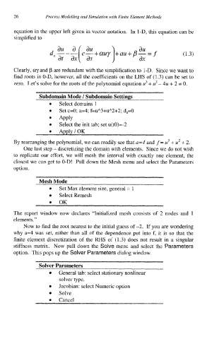
Subdomain Mode I Subdomain Settings
Select domains 1
Set c=O; a=4; f=uA3+uA2+2; d,=O
APPIY
Select the init tab; set u(tO)=-2

By rearranging the polynomial, we can readily see that a=4 and f = u3 + u2 + 2.
One last step - discretizing the domain with elements. Since we do not wish
to replicate our effort, we will mesh the interval with exactly one element, the
closest we can get to 0-D! Pull down the Mesh menu and select the Parameters
option.

Mesh Mode
Set Max element size, general = 1
Select Remesh
OK

The report window now declares “Initialized mesh consists of 2 nodes and 1
elements.”
Now to find the root nearest to the initial guess of -2. If you are wondering
why a=4 was set, rather than all of the dependence put into f, it is so that the
finite element discretization of the RHS of (1.3) does not result in a singular
stiffness matrix. Now pull down the Solve menu and select the Parameters
option. This pops up the Solver Parameters dialog window.

Solver Parameters
General tab: select stationary nonlinear
solver type.
Jacobian: select Numeric option
Solve
Cancel