Page 38 - Process Modelling and Simulation With Finite Element Methods

FEMLAB and the Basics ofNumerica1 Analysis 25

1.2.1 Root finding: A simple application of the FEMLAB nonlinear solver

As implied in the previous section, root finding is a “O-D” activity, at least in
ternis of the spatial-temporal dependence of the solution vector of unknowns, u,
which can be a multi-dimensional vector. FEMLAB does not have a “O-D”
application mode, so we must improvise in l-D. This has the undesirable feature
that we will unnecessarily solve the problem redundantly at several points in
space. Given the small size of the problem, the efficiency of FEMLAB coding,
and the speed of modem microprocessors, this causes no guilt whatsoever!

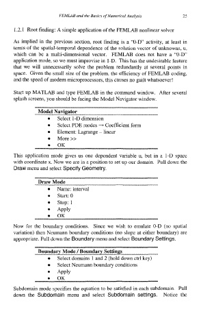
Start up MATLAB and type FEMLAB in the command window. After several
splash screens, you should be facing the Model Navigator window.

Model Navigator
Select 1-D dimension
Select PDE modes + Coefficient form
Element: Lagrange - linear
More >>
OK

This application mode gives us one dependent variable u, but in a l-D space
with coordinate x. Now we are in a position to set up our domain. Pull down the
Draw menu and select Specify Geometry.

Draw Mode
Name: interval
Start: 0
stop: 1
Apply
OK
Now for the boundary conditions. Since we wish to emulate O-D (no spatial
variation) then Neumann boundary conditions (no slope at either boundary) are
appropriate. Pull down the Boundary menu and select Boundary Settings.

Boundary Mode J Boundary Settings
Select domains 1 and 2 (hold down ctrl key)
Select Neumann boundary conditions
. APPlY

Subdomain mode specifies the equation to be satisfied in each subdomain. Pull
down the Subdomain menu and select Subdomain settings. Notice the