Page 43 - Process Modelling and Simulation With Finite Element Methods

30 Process Modelling and Simulation with Finite Element Methods

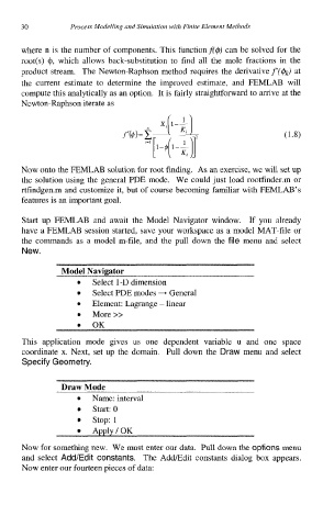
where n is the number of components. This functionf($) can be solved for the
root(s) @, which allows back-substitution to find all the mole fractions in the
product stream. The Newton-Raphson method requires the derivative f(&) at
the current estimate to determine the improved estimate, and FEMLAB will
compute this analytically as an option. It is fairly straightforward to arrive at the
Newton-Raphson iterate as

Now onto the FEMLAB solution for root finding. As an exercise, we will set up
the solution using the general PDE mode. We could just load ro0tfinder.m or
rtfindgen.m and customize it, but of course becoming familiar with FEMLAB’s
features is an important goal.

Start up FEMLAB and await the Model Navigator window. If you already
have a FEMLAB session started, save your workspace as a model MAT-file or
the commands as a model m-file, and the pull down the file menu and select
New.

Model Navigator
0 Select 1-D dimension
Select PDE modes + General
Element: Lagrange - linear
More >>
0
0 OK
This application mode gives us one dependent variable u and one space
coordinate x. Next, set up the domain. Pull down the Draw menu and select
Specify Geometry.

Draw Mode
Name: interval
Start: 0
stop: 1
Apply/OK

Now for something new. We must enter our data. Pull down the options menu
and select Add/Edit constants. The AddEdit constants dialog box appears.
Now enter our fourteen pieces of data: