Page 45 - Process Modelling and Simulation With Finite Element Methods

32 Process Modelling and Simulation with Finite Element Methods

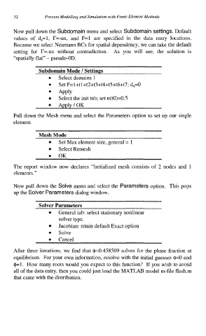
Now pull down the Subdomain menu and select Subdomain settings. Default
values of d,=l, T=-ux, and F=l are specified in the data entry locations.
Because we select Neumann BCs for spatial dependency, we can take the default
setting for T=-ux without contradiction. As you will see, the solution is
“spatially flat” - pseudo-OD.

Subdomain Mode I Settings
0 Select domains 1
0 Set F=l+tl+t2+t3+t4+t5+t6+t7; d,=O
Apply
Select the init tab; set u(t0)=0.5
Apply/OK

Pull down the Mesh menu and select the Parameters option to set up our single
element.

Mesh Mode
Set Max element size, general = 1
Select Remesh

0 OK
The report window now declares “Initialized mesh consists of 2 nodes and 1
elements.”

Now pull down the Solve menu and select the Parameters option. This pops
up the Solver Parameters dialog window.

Solver Parameters
General tab: select stationary nonlinear
solver type.
Jacobian: retain default Exact option
Solve

After three iterations, we find that $=0.458509 solves for the phase fraction at
equilibrium. For your own information, resolve with the initial guesses $=O and
@=1. How many roots would you expect to this function? If you wish to avoid
all of the data entry, then you could just load the MATLAB model m-file flash.m
that came with the distribution.