Page 48 - Process Modelling and Simulation With Finite Element Methods

FEMLAB und the Basics ofNumerica1 Analysis 35

should we stop? Well, there is more programming work for higher order
methods, so our time is a consideration. But intrinsically, functions may not be
very smooth in their k-th derivative that we are estimating. It is possible that in
increasing the “accuracy of the approximation”, the round-off error of higher
derivative terms so estimated becomes appreciable. If that is the case, with each
successive step, the error may grow rapidly. This implies that higher order
methods are less stable than lower order methods. The common choice for
integrating ODES is to use a fourth order Runge-Kutta method. This is fairly
compact to programme, gives good accuracy, and typically has good stability
character.

Other methods
There are two other famous problems in numerical integration that need
particular programming attention:
Numerical Instability. Suppose your integration diverges to be very far from
known test-cases, even with a high order accuracy method. Then it is likely that
your method is numerically unstable. You can cut down your step size and
eventually achieve numerical stability. However, this means a longer
calculation. If you are computing a great many such integrations and the
slowness really bothers you, try a semi-implicit method like predictor-corrector
schemes.
Stiff Systems. Stiff systems usually have two widely disparate length or time
scales on which physical mechanisms occur. Stiff systems may have “numerical
instability” of the explosive sort mentioned above, or they may have non-
physical oscillations. Try the book of Gear [2] for a recipe to treat stiff systems.

1.3.1 Numerical integration: A simple example
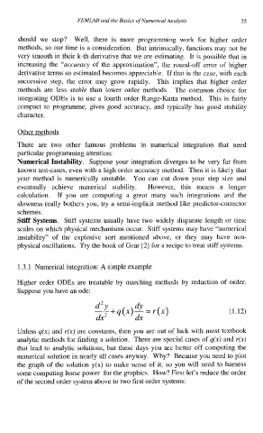
Higher order ODES are treatable by marching methods by reduction of order.
Suppose you have an ode:
-+q(x)-= dY +)
Y
d2
dx dx (1.12)
Unless q(x) and r(x) are constants, then you are out of luck with most textbook
analytic methods for finding a solution. There are special cases of q(x) and r(x)
that lead to analytic solutions, but these days you are better off computing the
numerical solution in nearly all cases anyway. Why? Because you need to plot
the graph of the solution y(x) to make sense of it, so you will need to harness
some computing horse power for the graphics. How? First let’s reduce the order
of the second order system above to two first order systems: