Page 46 - Process Modelling and Simulation With Finite Element Methods

FEMLAB and the Basics of Numerical Analysis 33

Exercises:

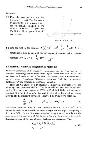
1.1 Find the root of the equation 6
f(u) = ueu - 1 = 0. This function is 5~
transcendental, which means that it 4~
has no analytic solution in the 3~
rational numbers. If you use 2~
Coefficient Mode, put c=l to aid li
covergence

1
2
5
3
1.2 Find the roots of the equation f (u)=u -3u +-u--=o. As this
2 2
function is a cubic polynomial, there is an analytic solution in the irrational
1 1
numbers, u=l, u=l--, u=l+-.
Jz Jz
1.3 Method 2: Numerical Integration by Marching
Numerical integration is the mainstay of numerical analysis. The first duty of
scientific computing before there were digital computers were to fill the
handbooks with tables of special functions, nearly all of which were solutions to
special classes of ordinary differential equations. And the computational
methodology? One-dimensional numerical integration.
There are two classes of I-D integration: initial value problems (IVP) and
boundary value problems (BVP). The latter will be considered in the next
section. The easiest to integrate are IVPs, as if all the initial conditions are all
specified at a point, it is straightforward to step along by small increments
according to the local first derivative. Clearly, if the ODE is first order, i.e.
dY
-=f (t), (1.9)
dt
The second statement in (1.9) is true exactly in the limit of At + 0. It is
termed the Euler method and is the most straight-forward way of integrating a
first order ODE. In one dimension, you simply step forward according to the
local value of the derivative off at the point (xn,yn), where n refers to the n-th
discretization step of the interval upon which you are integrating. Thus,

(1.10)
xn+l = x, + h