Page 50 - Process Modelling and Simulation With Finite Element Methods

FEMLAB and the Basics of Numerical Analysis 31

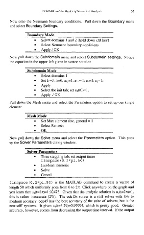
Now onto the Neumann boundary conditions. Pull down the Boundary menu
and select Boundary Settings.

Boundary Mode
Select domains 1 and 2 (hold down ctrl key)
Select Neumann boundary conditions
Apply/OK
Now pull down the Subdomain menu and select Subdomain settings. Notice
the equation in the upper left given in vector notation.
Subdomain Mode
Select domains 1
Set f1=0; f2=O; a12=l; aZ1=-l; cl=l; c2=l;
APPlY
Select the init tab; set u,(tO)=l.
Apply /OK

Pull down the Mesh menu and select the Parameters option to set up our single
element.

Mesh Mode
Set Max element size, general = 1
0
Select Remesh
OK
Now pull down the Solve menu and select the Parameters option. This pops
up the Solver Parameters dialog window.

Solver Parameters
Time-stepping tab: set output times
linspace (0,2*pi, 50)
Jacobian: numeric
0 Solve
0 Cancel
linspace (0,2*pi, 50) is the MATLAB command to create a vector of
length 50 which uniformly goes from 0 to 27~ Click anywhere on the graph and
you learn that ul(t=2n)=l .02475. Given that the analytic solution is u,(t=2~)=1,
this is rather inaccurate (2%). The odel5s solver is a stiff solver with low to
medium accuracy. ode45 has the best accuracy of the suite of solvers, but is for
non-stiff systems. It gives u1(t=6.29)=0.99994, which is pretty good. Greater
accuracy, however, comes from decreasing the output time interval. If the output